Attachment D - Nonresponse bias report
Attachment D - Nonresponse bias report.doc
Evaluation of the Community Healthy Marriage Initiative -- Impact Evaluation - Wave 2
Attachment D - Nonresponse bias report
OMB: 0970-0322
Attachment D
Analysis of Nonresponse Bias—Survey Wave 1
Evaluation of the Community Healthy Marriage Initiative
October 2008
Analysis of Nonresponse Bias—Survey Round 1: Evaluation of the Community Healthy Marriage Initiative
Report
Prepared for
Alan Yaffe
Office of Planning, Research and Evaluation
Administration for Children and Families
U.S. Department of Health and Human Services
370 L’Enfant Promenade, SW
Washington, DC 20447
Prepared by
701 13th Street, NW, Suite 750
Washington, DC 2005-3967
RTI Project Number 08957
Contents
Section Page
1. Background 1
2. Response Rates 3
3. Nonresponse Bias Analysis 5
3.1 Interpreting the Graph for the Frame Variables 5
3.2 Cleveland 8
3.2.1 Frame Variables 8
3.2.1.1 Access to CHMI Provider 8
3.2.1.2 Age Group Category 9
3.2.2 Level of Effort 10
3.2.2.1 Employed 10
3.2.2.2 Stable Relationship 10
3.3 Dallas 12
3.3.1 Frame Variables 12
3.3.1.1 Access to CHMI Provider 12
3.3.1.2 Age Group Category 13
3.3.1.3 Race Category 13
3.3.2 Level of Effort 14
3.3.2.1 Employed 15
3.3.2.2 Stable Relationship 15
3.4 Fort Worth 16
3.4.1 Frame Variables 16
3.4.1.1 Access to CHMI Provider 16
3.4.1.2 Age Group Category 17
3.4.1.3 Race Category 18
3.4.2 Level of Effort 19
3.4.2.1 Employed 19
3.4.2.2 Stable Relationship 19
3.5 Kansas City 21
3.5.1 Frame Variables 21
3.5.1.1 Access to CHMI Provider 21
3.5.1.2 Age Group Category 22
3.5.2 Level of Effort 22
3.5.2.1 Employed 23
3.5.2.2 Stable Relationship 23
3.6 Milwaukee 24
3.6.1 Frame Variables 24
3.6.1.1 Access to CHMI Provider 24
3.6.1.2 Age Group Category 24
3.6.2 Level of Effort 26
3.6.2.1 Employed 26
3.6.2.2 Stable Relationship 26
3.7 Saint Louis 27
3.7.1 Frame Variables 27
3.7.1.1 Access to CHMI Provider 27
3.7.1.2 Age Group Category 28
3.7.2 Level of Effort 29
3.7.2.1 Employed 29
3.7.2.2 Stable Relationship 29
4. Conclusion 31
Appendixes
A: Response Rates for Access to CHMI Provider, Age Category, and Race Category by CHMI Site A-1
B: Statistical Tests Related to the Disposition B-1
C: Employment and In Stable Relationship by CHMI Site and Stratification Variable Categories C-1
List of Exhibits
Number Page
1. Response Rates—Overall and By CHMI Site 3
List of Graphs
Number Page
1 Strata Weighted Percentages by Disposition 7
2 Strata Weighted Percentages for Access to CHMI Providers Category by Disposition Category for Cleveland 9
3 Strata Weighted Percentages for Age Group Category by Disposition Category for Cleveland 9
4 Proportion Employed by Number of Contacts Group for Cleveland 11
5 Proportion in Stable Relationship by Number of Contacts Group for Cleveland 11
6 Strata Weighted Percentages for Access to CHMI Providers Category by Disposition Category for Dallas 12
7 Strata Weighted Percentages for Age Group Category by Disposition Category for Dallas 13
8 Strata Weighted Percentages for Race by Disposition Category for Dallas 13
9 Proportion Employed by Number of Contacts Group for Dallas 15
10 Proportion in Stable Relationship by Number of Contacts Group for Dallas 15
11 Strata Weighted Percentages for Access to CHMI Providers Category by Disposition Category for Fort Worth 16
12 Strata Weighted Percentages for Age Group Category by Disposition Category for Fort Worth 18
13 Strata Weighted Percentages for Race by Disposition Category for Fort Worth 19
14 Proportion Employed by Number of Contacts Group for Fort Worth 20
15 Proportion in Stable Relationship by Number of Contacts Group for Fort Worth 20
16 Strata Weighted Percentages for Access to CHMI Providers Category by Disposition Category for Kansas City 21
17 Strata Weighted Percentages for Age Group Category by Disposition Category for Kansas City 22
18 Proportion Employed by Number of Contacts Group for Kansas City 23
19 Proportion in Stable Relationship by Number of Contacts Group for Kansas City 23
20 Strata Weighted Percentages for Access to CHMI Providers Category by Disposition Category for Milwaukee 24
21 Strata Weighted Percentages for Age Group Category by Disposition Category for Milwaukee 25
22 Proportion Employed by Number of Contacts Group for Milwaukee 26
23 Proportion in Stable Relationship by Number of Contacts Group for Milwaukee 27
24 Strata Weighted Percentages for Access to CHMI Providers Category and Disposition Category for Saint Louis 27
25 Strata Weighted Percentages for Age Group Category by Disposition Category for Saint Louis 29
26 Proportion Employed by Number of Contacts Group for Saint Louis 30
27 Proportion in Stable Relationship by Number of Contacts Group for Saint Louis 30
List of Tables
Number Page
1. Strata Weighted Percentages by Disposition 6
2. Effect of Overall Adjustment Factor 31
3. Effect of Stratum Level Adjustment Factors 32
1. Background
The Office of Family Assistance, Administration for Children and Families, is funding demonstration programs to support healthy marriage, improve child well-being, and increase the financial security of children in low-income communities. Among those demonstrations, the Community Healthy Marriage Initiative (CHMI) programs seek to increase the number of healthy marriages and change the norms in the communities where they operate to be more supportive toward healthy marriage. The primary goal of the CHMI evaluation is to analyze the CHMI programs’ effects on a number of outcomes, including marital and household status, attitudes about marriage and relationships, quality of relationships and marriages, and child well-being. The evaluation focuses on CHMI programs in Dallas, Milwaukee, and St. Louis, and will examine how effective these programs are in saturating their communities with marriage services and messaging, as well as how much the services and messaging affected behavioral outcomes and attitudes. The evaluation incorporates a statistical analysis of household survey data in these sites as well as in the matched comparison sites, Fort Worth, Cleveland, and Kansas City. Three rounds of primary data collection are planned to correspond with program implementation at early, intermediate, and late stages.
The Round 1 survey (or baseline survey) was conducted between October 2007 and April 2008. The survey collected data from adults ages 18-49 in the treatment and comparison communities. In the first stage of sample selection, RTI purchased address lists from the United States Postal Service of all households in the sampling areas. This sampling frame was stratified by age, access to a CHMI provider (defined by geographic proximity to a CHMI program), and race/ethnicity (for two sites only). The 13,000 selected households were screened for the number of eligible residents, and households were classified as eligible, ineligible, or unknown eligibility (in cases where screeners could not be completed). In the second-stage of sample selection, a household member was selected from among those eligible, and selected respondents were classified as either eligible and completed an interview or eligible and did not complete an interview. Thus, nonresponse occurred at both the screening phase and the interview phase.
Virtually all surveys experience some type of nonresponse. Nonresponse can occur when no information on the sampled unit is collected, called unit nonresponse, or when only partial information is collected, that is, some questions are not answered, called item nonresponse. In either case, estimates of population characteristics from the survey data have the potential for bias when not all sample members are interviewed. In this report, we explore the potential for nonresponse bias in the CHMI Round 1 survey. Our investigation includes (1) an evaluation of nonresponse rates, (2) a comparison of respondents and nonrespondents, and (3) a comparison of key analytic variables based on the level of effort, or the number of contact attempts made. Results from this analysis were used to inform the Round 1 weighting process and, in future rounds, will inform the allocation of interviewing resources to reduce the potential for nonresponse bias.
2. Response Rates
For Round 1, the overall weighted response rate was 63.18 percent, with response rates ranging from a low of 60.27 percent in Milwaukee to a high of 67.77 percent in Kansas City. The overall unweighted response rate was similar, 63.88 percent. Unweighted response rates are based on simple counts and weighted response rates are based on the design weight. The response rate is the product of the contact rate and the cooperation rate. The contact rate “measures the proportion of all cases in which some responsible member of the housing unit was reached by the survey,”1 and the cooperation rate “is the proportion of all cases interviewed of all eligible units ever contacted.”2 Exhibit 1 shows, overall and by CHMI site, the unweighted and weighted contact rates, cooperation rates, and response rates.
Exhibit 1. Response Rates—Overall and By CHMI Site
CHMI Site |
Unweighted Percent |
Weighted Percent |
||||
Contact Ratea |
Cooperation Rateb |
Response Ratec |
Contact Ratea |
Cooperation Rateb |
Response Ratec |
|
All |
79.58 |
80.27 |
63.88 |
79.80 |
79.17 |
63.18 |
Cleveland, OH |
78.10 |
81.61 |
63.74 |
77.83 |
81.38 |
63.33 |
Dallas, TX |
87.65 |
71.04 |
62.26 |
88.02 |
70.15 |
61.75 |
Ft. Worth, TX |
81.60 |
76.78 |
62.65 |
81.50 |
76.70 |
62.51 |
Kansas City, MO |
80.42 |
84.22 |
67.73 |
80.48 |
84.21 |
67.77 |
Milwaukee, WI |
73.82 |
83.62 |
61.73 |
72.61 |
83.00 |
60.27 |
St. Louis, MO |
77.01 |
86.44 |
66.57 |
76.81 |
84.55 |
64.94 |
a Contact rates were calculated using The American Association of Public Opinion Research (AAPOR) CON2 formula.3
b Cooperation rates were calculated using the AAPOR COOP1 formula.4
c Response rates were calculated using the AAPOR RR3 formula,5 which is equal to CON2 * COOP1.
Because the CHMI overall weighted response rate was less than 80 percent, we adhered to Guideline 3.2.9 from the Office of Management and Budget’s Standards and Guidelines for Statistical Surveys. This Guideline states, “Given a survey with an overall unit response rate of less than 80 percent, conduct an analysis of nonresponse bias using unit response rates defined above, with an assessment of whether the data are missing completely at random.”6 This report presents the results of our nonresponse bias analysis.
Although response rates may be an indicator of the potential for nonresponse bias, they are not a good predictor of nonresponse bias by themselves. The focus on response rates can be misleading because nonresponse bias analysis is for a specific statistic, not the survey in general. Consequently, we applied multiple methods of detecting nonresponse bias.
Appendix A contains information about subgroup response rates not covered in this report to investigate differential nonresponse by subgroup that may also lead to biased estimates.
3. Nonresponse Bias Analysis
In this section, we analyze variables that are available on the sampling frame, specifically, variables that were used to construct the sampling strata, and are thought to be associated with outcomes of interest. The variables were access to CHMI provider, age, and race/ethnicity. Hereafter, the race/ethnicity variable will be referred to as the race variable. Appendix C contains tables that validate our initial assumption that stratification variables are associated with outcomes of interest.
In addition to the stratification variables, we also examine the level of effort to contact the selected households in relation to two key analytic variables: employment status and relationship status (stable or not).
3.1 Interpreting the Graph for the Frame Variables
To analyze the variables available on the sampling frame, we used graphical techniques as well as statistical tests. The graphical investigation consisted of a simple plot for the analysis. The statistical tests were Chi-squared tests of independence for two categorical variables. The statistical tests tested the independence between the categories of the variable of interest and the categories of the disposition variable of the sampled cases, (that is, unknown eligibility, not eligible, eligible non-interview, and eligible completed interview). The statistical tests also tested the independence between the categories of the variable of interest and the categories for the known eligible, that is, eligible non-interviews and eligible completed interviews.
To analyze the plot, we visually compared the weighted relative sizes of the categories of the variable of interest across categories of the disposition variable. The weight used for these calculations was the design weight. If the weighted relative sizes of the categories of the variable of interest remained close to the reference value across categories of the disposition variable, we determined that the conditions leading to biased estimates were minimized. In this case, we would use one weighting adjustment factor for all categories of the variable of interest. Conversely, if the weighted relative sizes of the categories of the variable of interest deviated from the reference value across categories of the disposition variable, we determined that the conditions existed that could potentially produce biased estimates. In that case, we would use different weighting adjustment factors for each category of the variable of interest.
To make this concept more concrete, we provide an example using a table and a graph. Table 1 shows the percentage of the categories of the stratification variable, i.e., our variable of interest, by the categories of the disposition variable. The first row of data in the table is for the
Table 1. Strata Weighted Percentages by Disposition
|
Weighted Percentages |
|||
|
Stratum 1 |
Stratum 2 |
Stratum 3 |
Total |
|
|
|
|
|
Sample (Reference) |
50 |
35 |
15 |
100 |
|
|
|
|
|
Disposition |
|
|
|
|
Unknown Eligibility |
39 |
45 |
16 |
100 |
Not Eligible |
50 |
35 |
15 |
100 |
Eligible Non-interview |
61 |
25 |
14 |
100 |
Completed Interview |
55 |
30 |
15 |
100 |
distribution of the sample for the three strata and provides the reference information. That is, the distribution of the weighted sample is 50 percent in stratum one, 35 percent in stratum two, and 15 percent in stratum three. The remaining rows of data are for the disposition categories: unknown eligibility, not eligible, eligible non-interview, and eligible completed interview.
Ideally, we want the stratum disposition category values to be close to the stratum reference value for all strata. For example, stratum three has a stratum reference value of 15 percent. We would like to see all of the stratum three disposition category values close to this value. Because all the stratum three disposition category values are close to the stratum reference value, i.e., unknown eligibility 16 percent, not eligible 15 percent, eligible non-interview 14 percent, and eligible completed interview 15 percent, stratum three has the appropriate representation across the disposition categories. On the other hand, stratum one has a reference value of 50 percent and disposition category values that differ from it, i.e., unknown eligibility 39 percent, eligible non-interview 61 percent, and eligible completed interview 55 percent. Also, stratum two has a reference value of 35 percent and disposition category values that differ from it, i.e., unknown eligibility 45 percent, eligible non-interview 25 percent, and eligible completed interview 30 percent. Consequently, these strata do not have the appropriate representation across the disposition categories. Because not all of the strata remain close to their stratum reference values, we accounted for this variable in the weighting process by using different adjustment factors for each stratum so that each stratum represented its appropriate size, instead of a single adjustment for all strata.
Graph 1 is a visual representation of the data in Table 1. The lower horizontal axis shows the categories of the disposition variable. The left vertical axis shows the percentage for the strata. Recall that for each category of the disposition variable, the sum of the percentages
Graph 1. Strata Weighted Percentages by Disposition
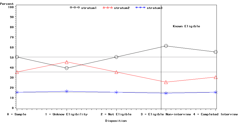
is 100 percent. That is, for each category of the disposition variable, the relative sizes of the strata are shown. The legend at the top of the plot identifies the three strata. Each stratum has a line in the plot with a different color and a different symbol. The horizontal lines represent the weighted relative sizes of the strata in the sample and provide a reference line for weighted relative sizes of the strata by the categories of the disposition variable. The weight used is the survey design weight, or the inverse of the probability of selection. The vertical line in the plot separates the categories before eligibility is known and ineligible cases from the eligible cases.
To analyze the plot of the three strata, we visually compared the weighted relative sizes of the strata across the categories of the disposition variable. On the left axis is the weighted percent of the strata from the sample, which provides the reference lines for the weighted percentage of the strata by disposition. As we move from left to right across the graph, we see:
1. Unknown eligibility
a. Stratum one—fewer cases than expected
b. Stratum two—more cases than expected
c. Stratum three—expected number of cases
2. Not eligible—All strata have the expected number of cases
3. Eligible non-interview
a. Stratum one—more cases than expected
b. Stratum two—fewer cases than expected
c. Stratum three—expected number of cases
4. Eligible completed interview
a. Stratum one—more cases than expected
b. Stratum two—fewer cases than expected
c. Stratum three—expected number of cases
Because of the deviations from the reference line for strata one and two for the unknown eligibility disposition, we included an unknown eligibility adjustment within stratum. Stratum one had a smaller adjustment factor than expected. Stratum two had a larger adjustment factor than expected. Stratum three had the expected adjustment factor.
Also, because of the deviations from the reference line for strata one and two for the eligible non-interview and eligible completed interview dispositions, we included a nonresponse adjustment within stratum. Stratum one had a larger adjustment factor than expected. Stratum two had a smaller adjustment factor than expected. Stratum three had the expected adjustment factor.
Note that if all of the strata had looked like stratum three, i.e., did not deviate from its expected size, no within stratum weight adjustments would have been necessary because all of the strata would have had their appropriate relative sizes. Instead, we would have used a single adjustment factor for all strata. Finally, note that the most important role of the unknown eligibility disposition may be in monitoring the effectiveness of the field staff to determine eligible cases. During data collection, significant deviations from the expected sizes for this category prompted a review of the protocols for gaining respondent cooperation.
Our primary interest was investigating nonresponse within the CHMI sites, and we anticipated that the sampling, weight adjustments, and poststratification would all be conducted within CHMI site. Therefore, all of the subsequent plots are grouped by specific CHMI site, and the weight used was the design weight. The statistical tests associated with different aspects of the plots are shown in Appendix B.
3.2 Cleveland
3.2.1 Frame Variables
For the frame variable investigation, we investigated the relationship between the stratification variables and the categories of the disposition variable. In Cleveland, the stratification variables were access to CHMI provider and age.
3.2.1.1 Access to CHMI Provider
Graph 2 is for the Cleveland site and contains the access to CHMI provider categories, i.e., high, medium, and low access.
Graph 2. Strata Weighted
Percentages for Access to CHMI Providers
Category by Disposition
Category for Cleveland
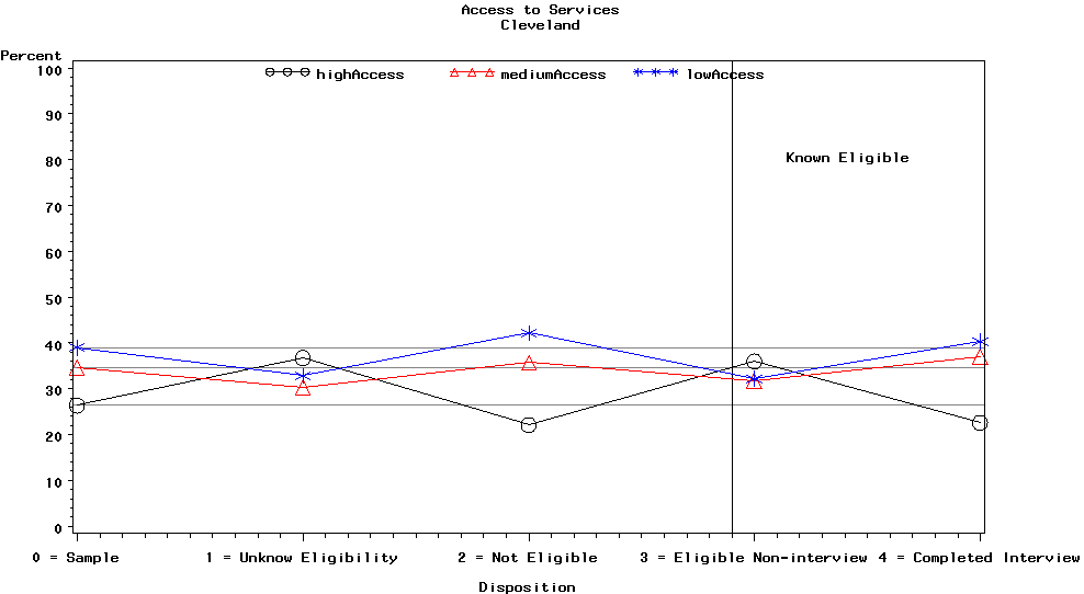
The most noticeable aspect of this plot is that the low access category had more unknown eligibility cases and eligible non-interviews than we would have expected, and slightly fewer eligible completed interviews than expected. Conversely, the medium access and low access categories had fewer unknown eligibility cases and eligible non-interviews than expected, and slightly more completed interviews than expected. The greater than expected relative size of the low access category in the unknown eligibility cases and eligible non-interviews category caused some concern because of the potential for nonresponse bias.
3.2.1.2 Age Group Category
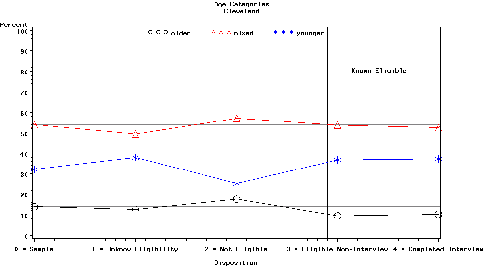
Graph 3 is for the Cleveland site and contains the categories of the age variable, i.e., older, mixed, and younger.
The most noticeable aspect of this plot is that the younger age category had more unknown eligibility cases than we would have expected, fewer ineligible cases, and more eligible non-interview cases than expected. However, having more unknown eligibility cases might not be too surprising because of the known difficulty of contacting younger people. The mixed-age category had fewer unknown eligibility cases than expected. The older age category had fewer eligible non-interviews and completed interviews than expected. The relative sizes of the mixed and younger categories for the unknown eligibility category, and the relative sizes of the younger and older age categories caused some concern because of the potential for nonresponse bias.
Graph 3. Strata Weighted
Percentages for Age Group
Category by Disposition Category for
Cleveland
3.2.2 Level of Effort
For the level of effort investigation, we analyzed only the completed interviews. This analysis investigated the relationship between the number of contact attempts and whether the respondent was employed, and the number of contact attempts and whether the respondent agreed or strongly agreed with the statement that their relationship with their partner was very stable.
3.2.2.1 Employed
Graph 4 is for the Cleveland site and contains the proportion employed by the categories for the number of contacts (1 contact, 2-4 contacts, 5-9 contacts, 10 or more contacts).
There is a trend that shows the proportion employed increases as the number of contacts increases. The p-value = 0.0040 for the linear trend test. Intuitively, this finding makes sense because people are at work and therefore more difficult to contact at home.
3.2.2.2 Stable Relationship
Graph 5 is for the Cleveland site and contains the proportion in a stable relationship by the categories for the number of contacts.
Graph 4. Proportion Employed by Number of Contacts Group for Cleveland

Graph 5. Proportion in Stable Relationship by Number of Contacts Group for Cleveland

There is a trend that shows the proportion in a stable relationship increases as the number of contacts increases. The p-value = 0.0144 for the linear trend test. Note that this trend is not always observed in the other sites.
3.3 Dallas
3.3.1 Frame Variables
For the frame variable investigation, we investigated the relationship between the stratification variables and the categories of the disposition variable. In Dallas, the stratification variables were access to CHMI provider, age, and race.
3.3.1.1 Access to CHMI Provider
Graph 6 is for the Dallas site and contains the access to CHMI provider categories, i.e., high, medium, and low access.
Graph 6. Strata Weighted Percentages for Access to CHMI Providers Category by Disposition Category for Dallas

The most noticeable aspect of this plot is that the high access category had more unknown eligibility cases than we would have expected and slightly fewer eligible non-interviews and eligible completed interviews than expected. The medium access category had fewer unknown eligibility cases than expected and fewer eligible non-interviews and eligible completed interviews than expected. The low access category had more eligible non-interviews and completed interviews than expected. The relative size of the low and medium access categories in the unknown eligibility category, and the relative size of all three access categories caused some concern because of the potential for nonresponse bias.
3.3.1.2 Age Group Category
Graph 7 is for the Dallas site and contains the categories of the age variable, i.e., older, mixed, and younger.
Graph 7. Strata Weighted
Percentages for Age Group
Category by Disposition Category for
Dallas

The most noticeable aspect of this plot is that the younger age category had more unknown eligibility cases than we would have expected and more eligible non-interview cases than expected. As mentioned, having more unknown eligibility cases might not be too surprising because of the known difficulty of contacting younger people. The mixed age category had fewer unknown eligibility cases than expected. The older age category had fewer eligible non-interviews than expected. The relative sizes of the mixed and younger categories for the unknown eligibility category, and the relative sizes of the younger and older age categories caused some concern because of the potential for nonresponse bias.
3.3.1.3 Race Category
Graph 8 is for the Dallas site and contains the categories of the race variable, i.e., Hispanic, white, and black. Race was used for only two CHMI sites, Dallas and Fort Worth.
Graph 8. Strata Weighted Percentages for Race by Disposition Category for Dallas
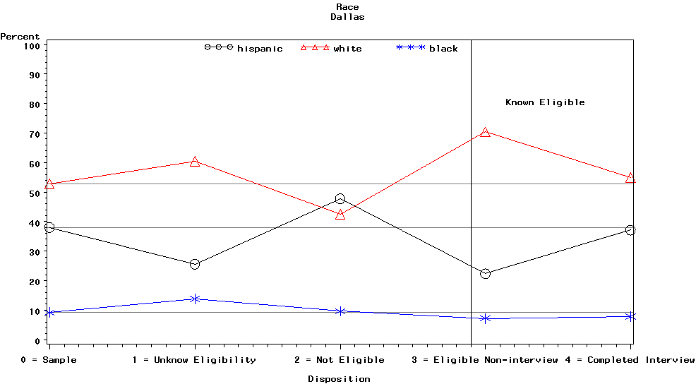
Notice that the relative size of the categories of the race variable in the sample is roughly equal to the relative size of the categories of the race variable for the completed interviews, but the race categories arrived at this in different ways. The black race category remained relatively close to its expected size across all of the disposition categories. The Hispanic and white race categories were different.
The Hispanic race category had fewer unknown eligibility cases, more ineligible cases, and significantly fewer eligible non-interview cases than expected. Conversely, the white race category had more unknown eligibility cases, fewer ineligible cases, and significantly more eligible non-interview cases than expected. These different paths from sample to completed interviews caused concern about the potential for nonresponse bias. If the unknown eligible cases were different from the eligible non-interviews and different from the respondents in relation to the analytic variables, the estimates may be biased.
3.3.2 Level of Effort
For the level of effort investigation, we analyzed only the completed interviews. This analysis investigated the relationship between the number of contact attempts and whether the respondent was employed, and the number of contact attempts and whether the respondent agreed or strongly agreed with the statement that their relationship with their partner was very stable.
3.3.2.1 Employed
Graph 9 is for the Dallas site and contains the proportion employed by the categories for the number of contacts.
Graph 9. Proportion Employed by Number of Contacts Group for Dallas
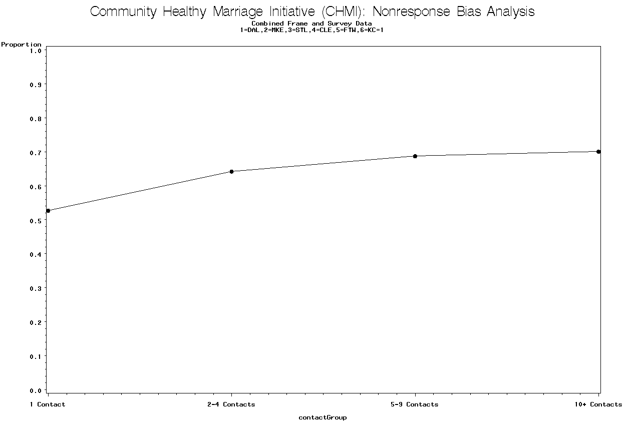
There is a trend that shows the proportion employed increases as the number of contacts increases. The p-value = 0.0160 for the linear trend test. This trend was observed in five of the six sites.
3.3.2.2 Stable Relationship
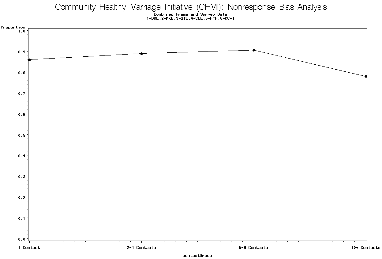
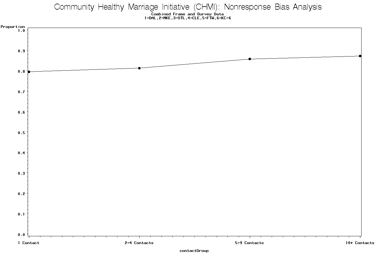
Graph 10 is for the Dallas site and contains the proportion in a stable relationship by the categories for the number of contacts.
There is not a trend that shows the proportion in a stable relationship changes as the number of contacts increases. The p-value = 0.4024 for the linear trend test.
Graph 10. Proportion in Stable
Relationship by
Number of Contacts Group for Dallas
3.4 Fort Worth
3.4.1 Frame Variables
For the frame variable investigation, we investigated the relationship between the stratification variables and the categories of the disposition variable. In Fort Worth, the stratification variables were access to CHMI provider, age, and race.
3.4.1.1 Access to CHMI Provider
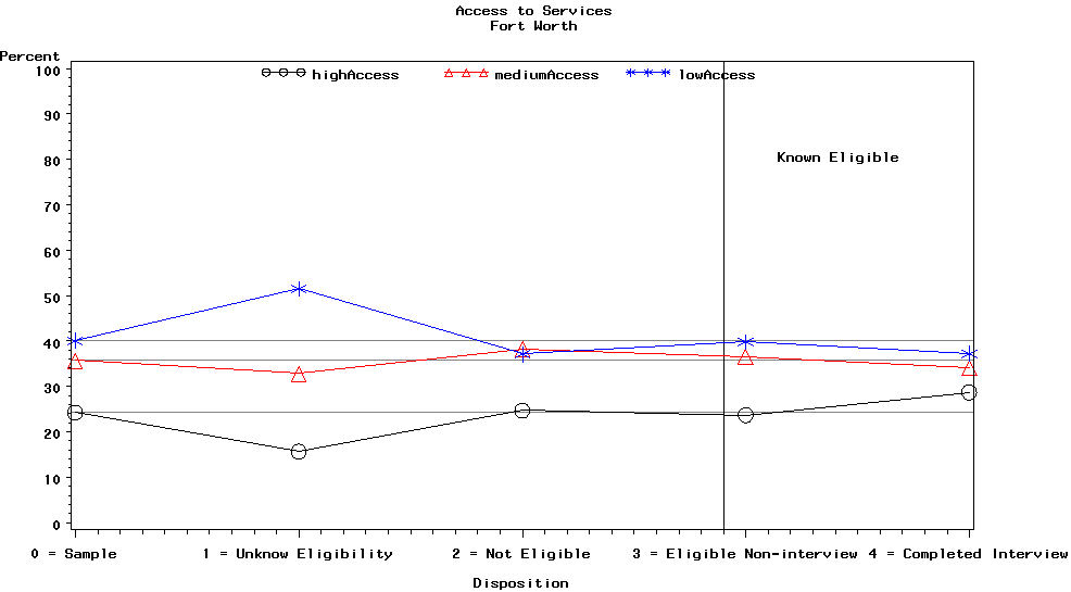
Graph 11 is for the Fort Worth CHMI site and contains the access to CHMI provider categories, i.e., high, medium, and low access.
In this plot, the low access category had significantly more unknown eligibility cases than we would have expected. Conversely, the medium access had slightly fewer unknown eligibility cases than expected, and the high access categories had significantly fewer unknown eligibility cases than expected. The spike in the relative size of the low access category in the unknown eligibility category caused some concern because of the potential for nonresponse bias.
Graph 11. Strata Weighted
Percentages for Access to CHMI Providers
Category by Disposition
Category for Fort Worth
3.4.1.2 Age Group Category
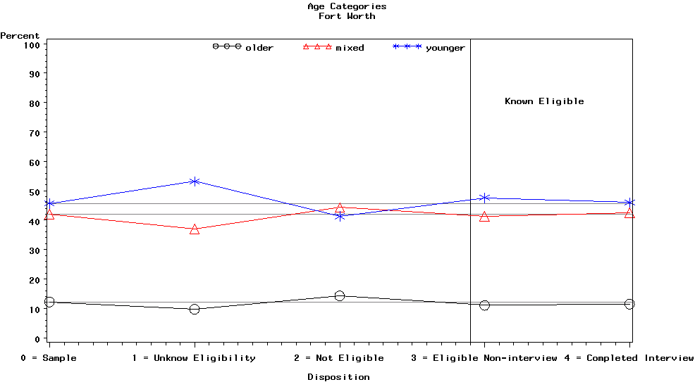
Graph 12 is for the Fort Worth site and contains the categories of the age variable, i.e., older, mixed, and younger.
In general, there is not as much movement in the relative sizes of the categories of the age variable across the categories of the disposition variable. Consequently, we had less concern about the potential for nonresponse bias than other variables where the relative sizes of the categories moved significantly away from the reference line.
The most noticeable aspect of this plot is that the younger age category had more unknown eligibility cases than we would have expected and slightly fewer ineligible cases than expected. We have observed this outcome with younger people in other sites. Conversely, the older and mixed age categories had fewer unknown eligibility cases than expected and slightly more ineligible cases than expected. All three age categories had about the expected number of completed interviews.
Graph 12. Strata Weighted
Percentages for Age Group
Category by Disposition Category for
Fort Worth
3.4.1.3 Race Category
Graph 13 is for the Fort Worth site and contains the categories of the race variable, i.e., Hispanic, white, and black. Race was used as a stratification variable in only two CHMI sites, Dallas and Fort Worth.
In Fort Worth, the relative size of the categories of the race variable in the sample is roughly equal to the relative size of the categories of the race variable for the completed interviews, but the race categories arrived at this in different ways. As we observed in Dallas, the black race category remained relatively close to its expected size across all of the disposition categories. The Hispanic and white race categories were different.
The Hispanic race category had fewer unknown eligibility cases, more ineligible cases, and significantly fewer eligible non-interview cases than expected. Conversely, the white race category had more unknown eligibility cases, fewer ineligible cases, and significantly more eligible non-interview cases than expected. These different paths from sample to completed interviews caused concern about the potential for nonresponse bias. If the unknown eligible cases were different from the completed non-interviews and different from the respondents in relation to the analytic variables, the estimates may be biased.
Graph 13. Strata Weighted
Percentages for Race by
Disposition Category for Fort Worth

3.4.2 Level of Effort
For the level of effort investigation, we analyzed only the completed interviews. This analysis investigated the relationship between the number of contact attempts and whether the respondent was employed, and the number of contact attempts and whether the respondent agreed or strongly agreed with the statement that their relationship with their partner was very stable.
3.4.2.1 Employed
Graph 14 is for the Fort Worth CHMI site and contains the proportion employed by the number of contacts.
There is a trend that shows the proportion employed increases as the number of contacts increases. The p-value = 0.0006 for the linear trend test.
3.4.2.2 Stable Relationship
Graph 15 is for the Fort Worth site and contains the proportion in a stable relationship by the categories for the number of contacts.
Graph 14. Proportion Employed by Number of Contacts Group for Fort Worth
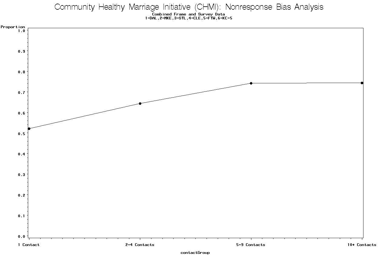
Graph 15. Proportion in Stable
Relationship by
Number of Contacts Group for Fort Worth

There is not a trend that shows the proportion in a stable relationship changes as the number of contacts increases. The p-value = 0.6568 for the linear trend test.
3.5 Kansas City
For the frame variable investigation, we investigated the relationship between the stratification variables and the categories of the disposition variable. In Kansas City, the stratification variables were access to CHMI provider and age.
3.5.1 Frame Variables
3.5.1.1 Access to CHMI Provider
Graph 16 is for the Kansas City site and contains the access to CHMI provider categories, i.e., high, medium, and low access.
Graph 16. Strata Weighted
Percentages for Access to CHMI Providers
Category by Disposition
Category for Kansas City
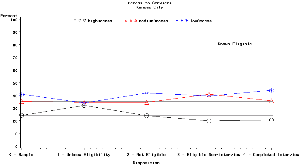
In this plot, the low access category had fewer unknown eligibility cases than expected and slightly more completed interviews than expected. On the other hand, the high access category had more unknown eligibility cases and eligible non-interviews than expected, and fewer eligible non-interviews and completed interviews than expected. The medium access category had more eligible non-interviews than expected. The relative sizes of the low and high access categories for the unknown eligibility cases, and the relative sizes of the medium and high access categories for the eligible non-interviews caused some concern because of the potential for nonresponse bias.
3.5.1.2 Age Group Category
Graph 17 is for the Kansas City site and contains the categories of the age variable, i.e., older, mixed, and younger.
Graph 17. Strata Weighted
Percentages for Age Group
Category by Disposition Category for
Kansas City
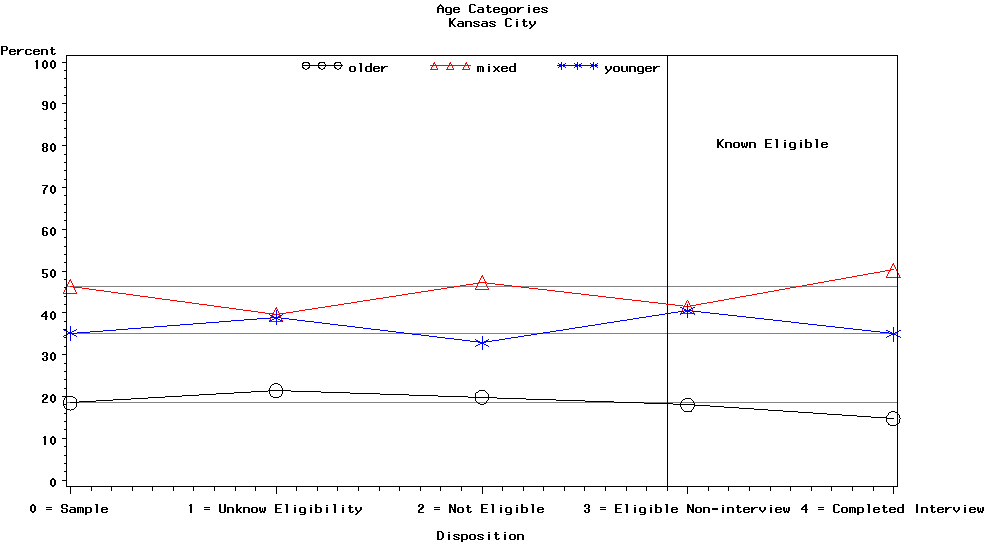
In Kansas City, the younger and older age categories had more unknown eligibility cases than we would have expected, and the mixed age category had fewer unknown eligibility cases than expected. The mixed age category had fewer eligible non-interview cases than expected, and the younger age category had more eligible non-interview cases than expected. Finally, the mixed age category had more completed interviews than expected, and the older age category had fewer completed interviews than expected. The relative sizes of the mixed and younger categories for the unknown eligibility category, and the relative sizes of the mixed and older age categories caused some concern because of the potential for nonresponse bias.
3.5.2 Level of Effort
For the level of effort investigation, we analyzed only the completed interviews. This analysis investigated the relationship between the number of contact attempts and whether the respondent was employed, and the number of contact attempts and whether the respondent agreed or strongly agreed with the statement that their relationship with their partner was very stable.
3.5.2.1 Employed
Graph 18 is for the Kansas City site and contains the proportion employed by the number of contacts.
Graph 18. Proportion Employed by Number of Contacts Group for Kansas City
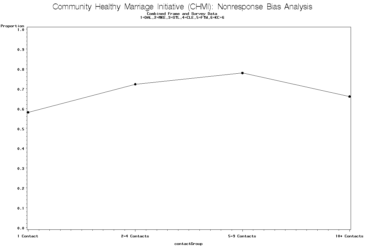
The trend shows that the proportion employed initially increases and then decreases as the number of contacts increases. The p-value = 0.3631 for the linear trend test does not indicate that there is a linear trend, but there may be a nonlinear relationship.
3.5.2.2 Stable Relationship
Graph 19 is for the Kansas City site and contains the proportion in a stable relationship by the number of contacts.
There is not a trend that shows the proportion in a stable relationship changes as the number of contacts increases. The p-value = 0.4320 for the linear trend test.
Graph 19. Proportion in Stable
Relationship by
Number of Contacts Group for Kansas City
3.6 Milwaukee
3.6.1 Frame Variables
For the frame variable investigation, we investigated the relationship between the stratification variables and the categories of the disposition variable. In Milwaukee, the stratification variables were access to CHMI provider and age.
3.6.1.1 Access to CHMI Provider
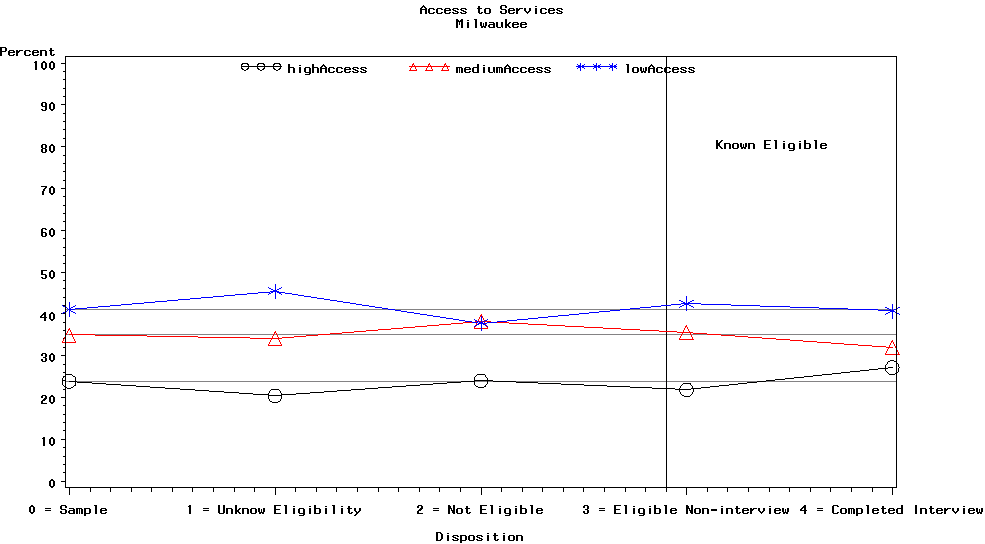
Graph 20 is for the Milwaukee site and contains the access to CHMI provider categories, i.e., high, medium, and low access.
In general, there is not as much movement in the relative sizes of the categories of the age variable across the categories of the disposition variable. Consequently, we had less concern about the potential for nonresponse bias than other variables where the relative sizes of the categories moved significantly away from the reference line.
3.6.1.2 Age Group Category
Graph 21 is for the Milwaukee site and contains the categories of the age variable, i.e., older, mixed, and younger.
Graph 20. Strata Weighted
Percentages for Access to CHMI Providers
Category by Disposition
Category for Milwaukee
Graph 21. Strata Weighted
Percentages for Age Group
Category by Disposition Category for
Milwaukee

The most noticeable aspect of this plot is that the mixed age category had more eligible non-interview cases and fewer completed interview cases than we would have expected. The younger age category had less eligible non-interview cases and more completed interview cases than we would have expected. The older age category had slightly fewer eligible non-interview cases and slightly fewer completed interview cases than expected. The relative sizes of all three age categories for the eligible non-interview category and completed interview category caused some concern because of the potential for nonresponse bias.
3.6.2 Level of Effort
For the level of effort investigation, we analyzed only the completed interviews. This analysis investigated the relationship between the number of contact attempts and whether the respondent was employed, and the number of contact attempts and whether the respondent agreed or strongly agreed with the statement that their relationship with their partner was very stable.
3.6.2.1 Employed
Graph 22 is for the Milwaukee site and contains the proportion employed by the number of contacts.
Graph 22. Proportion Employed by Number of Contacts Group for Milwaukee

There is a trend that shows the proportion employed increases as the number of contacts increases. The p-value = 0.0081 for the linear trend test.
3.6.2.2 Stable Relationship
Graph 23 is for the Milwaukee site and contains the proportion in a stable relationship by the categories for the number of contacts.
Graph 23. Proportion in Stable
Relationship by
Number of Contacts Group for Milwaukee

There is not a trend that shows the proportion in a stable relationship changes as the number of contacts increases. The p-value = 0.0576 for the linear trend test.
3.7 Saint Louis
3.7.1 Frame Variables
For the frame variable investigation, we investigated the relationship between the stratification variables and the categories of the disposition variable. In Saint Louis, the stratification variables were access to CHMI provider and age.
3.7.1.1 Access to CHMI Provider
Graph 24 is for the Saint Louis site and contains the access to CHMI provider categories, i.e., high, medium, and low access.
Graph 24. Strata Weighted
Percentages for Access to CHMI Providers
Category and
Disposition Category for Saint Louis
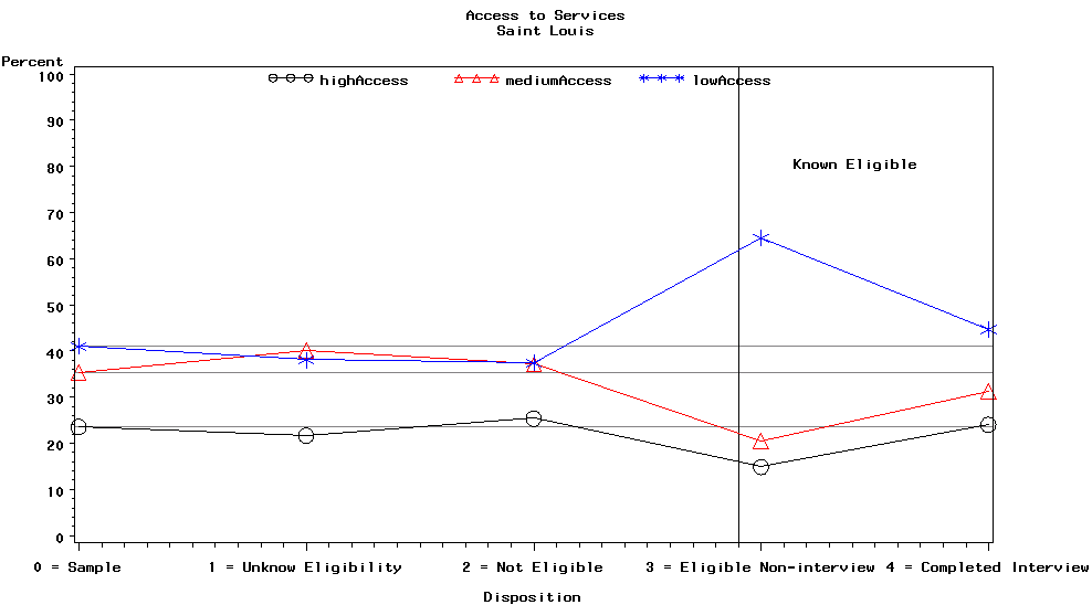
In this plot, the low access category had significantly more eligible non-interviews than expected and slightly more completed interviews than expected. Conversely, the medium access and low access categories had fewer eligible non-interviews than expected, and the medium access category had slightly fewer completed interviews than expected. The high access category had about the expected number of completed interviews. The spike in the relative size of the low access category in the eligible non-interviews category caused concern because of the potential for nonresponse bias.
3.7.1.2 Age Group Category
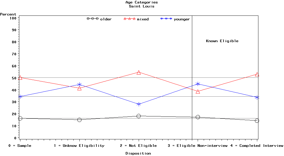
Graph 25 is for the Saint Louis site and contains the categories of the age variable, i.e., older, mixed, and younger.
The most noticeable aspect of this plot is that the younger age category had more unknown eligibility cases and eligible non-interview cases. The mixed age category had fewer unknown eligibility cases and eligible non-interview cases than expected. The relative sizes of mixed and younger age categories for the unknown eligibility category, and eligible non-interview category caused some concern because of the potential for nonresponse bias.
Graph 25. Strata Weighted
Percentages for Age Group
Category by Disposition Category for
Saint Louis
3.7.2 Level of Effort
For the level of effort investigation, we analyzed only the completed interviews. This analysis investigated the relationship between the number of contact attempts and whether the respondent was employed, and the number of contact attempts and whether the respondent agreed or strongly agreed with the statement that their relationship with their partner was very stable.
3.7.2.1 Employed
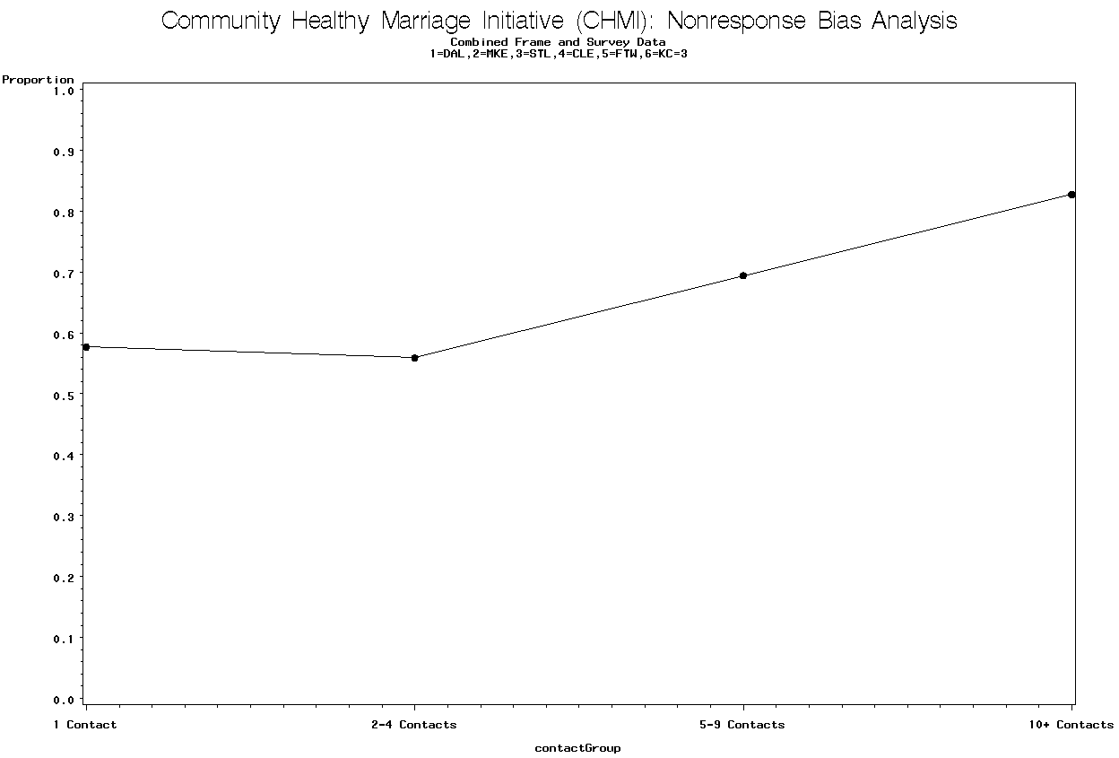
Graph 26 is for the Saint Louis site and contains the proportion employed by the number of contacts.
There is a trend that shows the proportion employed increases as the number of contacts increases. The p-value = 0.0000 for the linear trend test.
3.7.2.2 Stable Relationship
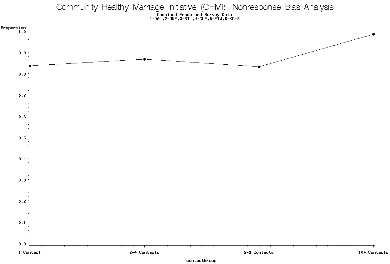
Graph 27 is for the St. Louis site and contains the proportion in a stable relationship by the number of contacts.
There is a trend that shows the proportion in a stable relationship increases as the number of contacts increases. The p-value = 0.0026 for the linear trend test.
Graph 26. Proportion Employed by Number of Contacts Group for Saint Louis
Graph 27. Proportion in Stable
Relationship by
Number of Contacts Group for Saint Louis
4. Conclusion
Based on the cumulative information from this investigation that indicated the potential for nonresponse bias existed, we included access to CHMI provider and age in the weighting process for all CHMI sites. For Dallas and Fort Worth, we also included race/ethnicity in the weighting process. For this survey round, we did not include the number of contacts in the weighting process because other variables capture some of the same variability in the analytic variables and the results related to the analytic variables were mixed, but we will monitor this situation for future rounds of weighting.
As a simplified example, the following two tables show why there may have been bias if we had not adjusted within the access to CHMI provider categories. We use Kansas City to illustrate. Recall that our assumption was that important analytic variables differed within the categories of access to CHMI provider; this assumption is supported by the empirical evidence. Both tables show the frame count, sum of the design weights for the sample, sum of the design weights for the known eligibility cases, the unknown eligibility adjustment factor, sum of the unknown eligibility adjusted weights for known eligibility cases, and the difference between the frame count and sum of the unknown eligibility adjusted weights. Table 2 shows the effect of an overall adjustment factor, and Table 3 shows the effect of access-level adjustment factors.
Table 2 shows that the overall adjustment factor would have created differences in the stratum frame counts and sum of the unknown eligibility adjusted weights that could have led to biased estimates.
Table 2. Effect of Overall Adjustment Factor
Access |
Frame |
Sample (Sum Design Weights) |
Known Eligibility (Sum Design Weights) |
Unknown Eligibility Adjustment Factor |
Known Eligibility (Sum Unknown Eligibility Adjusted Weights) |
Frame Minus Sum Unknown Eligibility Adjusted Weights |
High |
12,432 |
12,432 |
9,221 |
1.24 |
11,457 |
975 |
Medium |
18,082 |
18,082 |
14,642 |
1.24 |
18,192 |
-110 |
Low |
20,952 |
20,952 |
17,558 |
1.24 |
21,816 |
-864 |
Table 3 shows that the individual stratum-level adjustment factor matches the stratum frame counts and sum of the unknown eligibility adjusted weights. This approach minimized the potential for biased estimates.
Table 3. Effect of Stratum Level Adjustment Factors
Access |
Frame |
Sample (Sum Design Weights) |
Known Eligibility (Sum Design Weights) |
Unknown Eligibility Adjustment Factor |
Known Eligibility (Sum Unknown Eligibility Adjusted Weights) |
Frame Minus Sum Unknown Eligibility Adjusted Weights |
High |
12,432 |
12,432 |
9,221 |
1.35 |
12,432 |
0 |
Medium |
18,082 |
18,082 |
14,642 |
1.23 |
18,082 |
0 |
Low |
20,952 |
20,952 |
17,558 |
1.19 |
20,952 |
0 |
This example demonstrates the importance of weighting within the strata. In practice, we used the cross-classification of the access to CHMI provider, age, and race to create strata for making nonresponse adjustments. This deeper stratification created even larger deviations, for which we had to account. In a few instances, it was necessary to collapse some of the cross-classified strata. We believe that this weighting plan effectively minimized the potential for nonresponse bias in the variables (and their correlates) investigated in this report.
Appendix A: Response Rates for Access to CHMI Provider, Age Category, and Race Category by CHMI Site
Differential response rates across subgroups with different characteristics may result in nonresponse bias. The following tables examine access to CHMI provider, age, and race categories within CHMI sites. There was differential response among the different categories for all three variables. Consequently, we included these variables in the weighting process.
Table A1. Response Rates for CHMI Site by Access to CHMI Provider
CHMI Site |
Access to CHMI Provider |
||
Most Access (%) |
Medium Access (%) |
Low Access (%) |
|
Cleveland, OH |
50.62 |
67.34 |
68.75 |
Dallas, TX |
59.54 |
64.79 |
60.73 |
Ft. Worth, TX |
70.40 |
62.59 |
57.53 |
Kansas City, MO |
62.78 |
66.66 |
71.72 |
Milwaukee, WI |
65.76 |
59.70 |
57.45 |
St. Louis, MO |
70.66 |
65.70 |
62.12 |
Table A2. Response Rates for CHMI Site by Age Category
CHMI Site |
Age Category |
||
Older (%) |
Mixed (%) |
Younger (%) |
|
Cleveland, OH |
65.98 |
64.55 |
60.19 |
Dallas, TX |
64.52 |
63.96 |
58.97 |
Ft. Worth, TX |
65.93 |
64.61 |
59.70 |
Kansas City, MO |
62.92 |
72.14 |
64.43 |
Milwaukee, WI |
56.12 |
58.83 |
63.09 |
St. Louis, MO |
64.45 |
71.43 |
56.11 |
Table A3. Response Rates for CHMI Site by Access to CHMI Provider
CHMI Site |
Race Category |
||
More than 50% Black (%) |
More than 50% Hispanic (%) |
Other (%) |
|
Dallas, TX |
73.17 |
55.84 |
59.03 |
Ft. Worth, TX |
68.79 |
56.14 |
63.76 |
Appendix B: Statistical Tests Related to the Disposition
The chi-squared tests of independence for the categories of the access to CHMI provider variable and the categories of the disposition variable within CHMI site are located in Table B1. All of the tests were highly significant at the α = 0.05 level, indicating there is an association between the categories of the access to CHMI provider variable and disposition variable within CHMI site. We were sensitive to these associations in the weighting process because of the potential for nonresponse bias.
Table B1. Chi-squared Tests of Independence for the Access to CHMI Provider Categories and Disposition Categories within CHMI Site
CHMI Site |
Test |
DF |
Test Value |
P-value |
Cleveland |
ChiSq Wald F |
6 |
6.91 |
0.0000 |
Dallas |
ChiSq Wald F |
6 |
5.60 |
0.0000 |
Fort Worth |
ChiSq Wald F |
6 |
5.65 |
0.0000 |
Kansas City |
ChiSq Wald F |
6 |
3.47 |
0.0020 |
Milwaukee |
ChiSq Wald F |
6 |
2.90 |
0.0080 |
Saint Louis |
ChiSq Wald F |
6 |
5.88 |
0.0000 |
The chi-squared tests of independence for the categories of the access to CHMI provider variable and categories of the known eligibility cases within CHMI site are located in Table B2. Cleveland and Saint Louis were significant at the α = 0.05 level, indicating there is an association between the categories of the access to CHMI provider variable and the known eligibility cases within CHMI site. We were sensitive to these associations in the weighting process because of the potential for nonresponse bias.
Table B2. Chi-squared Tests of Independence for the Access to CHMI Provider Categories and Known Eligible Categories within CHMI Site
CHMI Site |
Test |
DF |
Test Value |
P-value |
Cleveland |
ChiSq Wald F |
2 |
4.07 |
0.0172 |
Dallas |
ChiSq Wald F |
2 |
0.25 |
0.7801 |
Fort Worth |
ChiSq Wald F |
2 |
0.97 |
0.3785 |
Kansas City |
ChiSq Wald F |
2 |
0.56 |
0.5725 |
Milwaukee |
ChiSq Wald F |
2 |
1.39 |
0.2487 |
Saint Louis |
ChiSq Wald F |
2 |
6.85 |
0.0011 |
The chi-squared tests of independence for the categories of the age variable and categories of the disposition variable within CHMI site are located in Table B3. All of the tests were significant at the α = 0.05 level, indicating there is an association between categories of the age variable and categories of the disposition variable within CHMI site. We were sensitive to these associations in the weighting process because of the potential for nonresponse bias.
Table B3. Chi-squared Tests of Independence for the Age Categories and Disposition Categories within CHMI Site
CHMI Site |
Test |
DF |
Test Value |
P-value |
Cleveland |
ChiSq Wald F |
6 |
7.89 |
0.0000 |
Dallas |
ChiSq Wald F |
6 |
2.27 |
0.0339 |
Fort Worth |
ChiSq Wald F |
6 |
2.49 |
0.0206 |
Kansas City |
ChiSq Wald F |
6 |
3.07 |
0.0053 |
Milwaukee |
ChiSq Wald F |
6 |
3.27 |
0.0033 |
Saint Louis |
ChiSq Wald F |
6 |
8.30 |
0.0000 |
The chi-squared tests of independence for the categories of the age variable and the known eligibility cases within CHMI site are located in Table B4. Milwaukee and Saint Louis were significant at the α = 0.05 level, indicating there is an association between categories of the age variable and the known eligibility cases within CHMI site. We were sensitive to these associations in the weighting process because of the potential for nonresponse bias.
Table B4. Chi-squared Tests of Independence for the Age Categories and Known Eligible Categories within CHMI Site
CHMI Site |
Test |
DF |
Test Value |
P-value |
Cleveland |
ChiSq Wald F |
2 |
0.05 |
0.9488 |
Dallas |
ChiSq Wald F |
2 |
0.73 |
0.4800 |
Fort Worth |
ChiSq Wald F |
2 |
0.07 |
0.9316 |
Kansas City |
ChiSq Wald F |
2 |
1.49 |
0.2264 |
Milwaukee |
ChiSq Wald F |
2 |
4.40 |
0.0176 |
Saint Louis |
ChiSq Wald F |
2 |
3.63 |
0.0266 |
The chi-squared tests of independence for the categories of the race variable and categories of the disposition within CHMI site are located in Table B5. All of the tests were significant at the α = 0.05 level, indicating there is an association between the categories of the race variable and the disposition variable within CHMI site. We were sensitive to these associations in the weighting process because of the potential for nonresponse bias.
Table B5. Chi-squared Tests of Independence for the Race Categories and Disposition Categories within CHMI Site
CHMI Site |
Test |
DF |
Test Value |
P-value |
Dallas |
ChiSq Wald F |
6 |
16.34 |
0.0000 |
Fort Worth |
ChiSq Wald F |
6 |
5.00 |
0.0000 |
The chi-squared tests of independence for the categories of the race variable and the known eligibility cases within CHMI site are located in Table B6. All of the tests were significant at the α = 0.05 level, indicating there is an association between the categories of the race variable and the known eligibility cases within CHMI site. We were sensitive to these associations in the weighting process because of the potential for nonresponse bias.
Table B6. Chi-squared Tests of Independence for the Age Categories and Known Eligible Categories within CHMI Site
CHMI Site |
Test |
DF |
Test Value |
P-value |
Dallas |
ChiSq Wald F |
2 |
11.36 |
0.0000 |
Fort Worth |
ChiSq Wald F |
2 |
5.19 |
0.0056 |
Appendix C: Employment and In Stable Relationship by CHMI Site and Stratification Variable Categories
These tables confirm our initial assumption that access to CHMI provider, age, and race are related to two important analytic variables, employment status and stable relationship status. In general, there were differential levels of employment and stable relationships across the different categories.
Table C1. Employment and In Stable Relationship by CHMI Site and Access to CHMI Provider Categories
CHMI Site |
Employed Proportion |
In Stable Relationship
Proportion |
||||
Most Access |
Medium Access |
Low Access |
Most Access |
Medium Access |
Low Access |
|
Cleveland, OH |
0.58 |
0.50 |
0.58 |
0.90 |
0.85 |
0.78 |
Dallas, TX |
0.61 |
0.66 |
0.60 |
0.90 |
0.85 |
0.88 |
Ft. Worth, TX |
0.61 |
0.61 |
0.67 |
0.90 |
0.85 |
0.88 |
Kansas City, MO |
0.77 |
0.63 |
0.64 |
0.79 |
0.75 |
0.88 |
Milwaukee, WI |
0.56 |
0.56 |
0.67 |
0.77 |
0.81 |
0.77 |
St. Louis, MO |
0.59 |
0.59 |
0.66 |
0.84 |
0.75 |
0.92 |
Table C2. Employment and In Stable Relationship by CHMI Site and Age Categories
CHMI Site |
Employed Proportion |
In Stable Relationship
Proportion |
||||
Older |
Mixed |
Younger |
Older |
Mixed |
Younger |
|
Cleveland, OH |
0.63 |
0.61 |
0.45 |
0.87 |
0.80 |
0.87 |
Dallas, TX |
0.66 |
0.62 |
0.61 |
0.95 |
0.88 |
0.86 |
Ft. Worth, TX |
0.69 |
0.65 |
0.60 |
0.89 |
0.89 |
0.86 |
Kansas City, MO |
0.67 |
0.69 |
0.62 |
0.87 |
0.84 |
0.74 |
Milwaukee, WI |
0.63 |
0.63 |
0.56 |
0.74 |
0.80 |
0.77 |
St. Louis, MO |
0.63 |
0.64 |
0.59 |
0.93 |
0.83 |
0.87 |
Table C3. Employment and In Stable Relationship by CHMI Site and Race Categories
CHMI Site |
Employed Proportion |
In Stable Relationship
Proportion |
||||
More than 50% Black |
More than 50% Hispanic |
Other |
More than 50% Black |
More than 50% Hispanic |
Other |
|
Dallas, TX |
0.63 |
0.60 |
0.71 |
0.84 |
0.89 |
0.97 |
Ft. Worth, TX |
0.60 |
0.66 |
0.63 |
0.87 |
0.86 |
0.92 |
1 The American Association of Public Opinion Research. 2008. Standard Definitions: Final Dispositions of Case Codes and Outcome Rates for Surveys. 5th edition. Lenexa, Kansas: AAPOR. Page 38.
2 AAPOR, page 36.
3 AAPOR, page 38.
4 AAPOR, page 36.
5 AAPOR, page 35.
6 Office of Management and Budget. 2006. Standards and Guidelines for Statistical Surveys. Washington, DC: OMB. Page 16.
| File Type | application/msword |
| File Title | Attachment D |
| Author | DHHS |
| Last Modified By | DHHS |
| File Modified | 2009-06-09 |
| File Created | 2009-06-09 |
© 2026 OMB.report | Privacy Policy