2363ssb01

One of the main issues in the study of vehicle emissions is the difficulty in acquiring representative results. Major challenges include the diversity of technology, the highly variable nature of emissions, the complexity and expense of measurement, difficulty in acquiring and retaining engines or vehicles, and the array of external variables that influence emissions, ranging from temperature to driver behavior. In combination, these factors tend to limit the numbers of vehicles that can be included in a given study. Limited sample sizes in combination with high variability make emissions data challenging to interpret.

Much research has shown that vehicle emissions tend to follow strongly skewed distributions, such as lognormal, Weibull or gamma distributions^¹^,^². Most vehicles are “clean,” with a relatively small number emitting at exceptionally “high” levels, and contributing inordinately to the total emissions loading. To capture representative results it is important that the entire distribution be sampled, including the upper percentiles in the right tail. However, the high-emitting vehicles are relatively rare, enough so that it is challenging for fully randomized sampling of the population as a whole to capture them in sufficient numbers to deliver representative averages.

The variability and skewed nature of emissions distributions complicate one of the most important analytic topics in emissions research, “emissions deterioration,” or the tendency of the average emissions levels to increase as vehicles age. This behavior is well documented^³, but remains difficult to study due to high variability. The sources of deterioration are complex, including general wear as well as failures in specific components. Analysis of available data shows that deterioration is expressed through a relatively small shift in the central portion of the distribution, accompanied by a larger and proportional spreading of the tail. These factors imply that accurate assessment of emissions deterioration requires represntative sampling across the entire age range.

The problem is difficult, in that some common approaches to sampling rare populations are not practical. No separate frames are available. High-emitting vehicles cannot be reliably isolated geographically, nor can they be exclusively associated with particular demographic groups. As an approach to capturing high-emitting vehicles, some form of screening would be valuable.

A technology is available that has potential to serve as a screening technique, known as “Infrared Long-path Photometry” or less formally as “remote-sensing.” It has been in use for over 25 years^⁴, for a variety of purposes, including general assessment of fleet emissions³, and evaluation of Inspection and Maintenance programs.^⁵^,^⁶ The instrument directs infrared (IR) and ultraviolet (UV) beams across the roadway between sources and detectors. When a vehicle travels through the beams, its exhaust plume intersects the beams, allowing spectroscopic measurements of exhaust constituents, including carbon monoxide (CO), hydrocarbons (HC), both by IR, and nitrogen oxide (NO), by UV. Some researchers have developed instrumentation designed to measure particulate-matter emissions.^⁷ The technique does not capture absolute measurements of emissions, but rather ratios of the constituents to exhaust CO₂ in the plume.

This technique fulfills criteria for a screening technique. It is relatively quick and inexpensive, allowing the rapid acquisition of large vehicle samples. It acquires a measurement of the vehicle’s emissions prior to sampling or recruitment without burdening the owner in any way.

The collection is a survey, to be conducted by the Office of Transportation and Air Quality (OTAQ) in the Office of Air and Radiation (OAR). This study will be designed to develop and test novel screening, sampling and measurement procedures. These approaches promise to substantially reduce the cost of exhaust emissions measurement as well as to improve the accuracy of resulting estimates.

An innovative feature of this project will be the use of roadside remote-sensing measurements to construct a pool of vehicles from which vehicles can be sampled for purposes of recruitment and measurement using portable emissions measurement systems (PEMS). The acquisition of remote-sensing measurements for hydrocarbons, carbon-monoxide, and oxides of nitrogen will provide an index of emissions for all vehicles prior to sampling and recruitment for more intensive measurement. The index is expected to facilitate recruitment of vehicles with an emphasis on high-emitting vehicles, and provide a means to appropriately relate measured vehicles to the target population.

Research questions for the project include:

Can remote-sensing be used as a reliable index of emissions across the range of emissions and vehicle age?
Is it feasible to measure start emissions using portable instruments?

When an engine is started, a large volume of fuel is injected into the cylinder to initiate ignition while the engine is cold and only the volatile gasoline components readily vaporize. This fuel results in an excess increment of emissions over that expected when the engine has come to operating temperature and the catalyst is functioning efficiently. Despite advances in engine technology, fuel control and emissions control, these “start” emissions remain a relatively high fraction of total emissions, due to the technical difficulties in controlling emissions while the engine is cold and the emissions control systems have not warmed up. Start emissions have been measured in the laboratory by repeating a pre-arranged test procedure under both cold and hot engine conditions and estimating the start increment as the difference of the two, as it is extremely difficult to distinguish “start emissions” from “running emissions” without the reference frame provided by replication. However, with the increasing importance of portable instruments, it is critical to develop or adapt techniques for measuring start emissions.

Can the emissions index used for recruitment also serve as a means to estimate potential non-response bias?

To the extent that the index serves as an efficient screening tool, it may also serve as a valuable tool to investigate potential non-response bias. The availability of an index of emissions for vehicles owned by non-responders may allow assessment of the key factor in non-response bias, namely, that response may be related to the parameter of interest, i.e., vehicle emissions.

How many “trips” do drivers make in a typical day, where a trip is defined as “key-on” to “key-off?” Does the number of trips/day differ between weekdays and weekends?

In this context, a trip begins when a driver turns the engine on and proceeds to a destination, and ends when they park and turn the engine off. As defined above, “start” emissions occur at the outset of a trip, and obviously, “running” emissions occur during the trip.

This data collection is a survey designed to estimate the exhaust emissions and usage of a sub-population of vehicles certified to selected certification standards, and having similar vehicle technology.

1(b) Key Variables

Variables to be surveyed or measured include:

Vehicle identifiers: License plate and Vehicle Identification Number
Vehicle description : make, model, model year, engine displacement, transmission type, engine family, and odometer reading
Vehicle usage and maintenance history
Exhaust gaseous emissions including CO₂, HC, CO and NOx, to be measured on a continuous “second-by-second” basis over a specified drive route
Exhaust particulate emissions to be measured on an aggregate basis over a specified drive route
Vehicle and engine operating parameters, including on-board diagnostic trouble codes, engine-coolant temperature, exhaust flow rate, engine speed, engine load, vehicle speed, oxygen sensors, air:fuel ratio, and global-positioning system coordinates.

1(c) Statistical Approach

We have selected a statistical approach for this effort for two reasons:

(1) While a census or partial census would be ideal, the effort and expense required is prohibitive.

(2) To meet the objectives for use of these data, it is necessary to draw valid and defensible inferences from sets of vehicles surveyed or measured to the vehicle population sampled. This requirement in itself rules out non-probabilistic approaches.

1(d) Feasibility

Obstacles to Participation. We do not anticipate substantial obstacles to participation. Participation does impose some burden for some potential participants, as they must modify their schedules to travel to and from the facility to drop off and pick up their vehicles. Thus, we anticipate that, in conjunction with incentives, solicitation will prove no more difficult than than in previous studies.

Availability of Funds. At present we expect to have adequate funds available to conduct the survey as designed. However, if funding shortfalls occur, we can take measures to reduce sampling costs. One possibility would be to reduce the number of vehicles in the study.

2.0 Survey Design

2(a) Target Population and Coverage

The target population is defined as the fleet of privately-owned gasoline-powered passenger cars and light-duty trucks certified to “Tier-2/Bin 5” or “LEV-II/LEV” standards. Light-duty trucks are trucks with gross vehicle weight ratings of less than 8,500 lbs. Passenger cars and light-duty trucks form the majority of the on-road motor vehicle fleet.

Vehicles certified to Bin-5 standards were introduced in model year 2004 and comprised approximately 70% of annual sales by 2007. Tier-2 standards apply to vehicles sold in states following Federal emissions standards, whereas the LEV-II program applies to vehicles certified for sale in California and states having adopted “California” standards since 2004. Some vehicles are certifed for sale in either Federal or “California” areas. Vehicles in both groups are certified to comparable standards, as shown in Table 1.

Coverage for this study will comprise the fleet of vehicles operating in the Detroit Metropolitan Statistical Area, Michigan. The Detroit-Ann Arbor-Flint Consolidated MSA includes the Michigan counties of Lapeer , Macomb, Monroe, Oakland , St. Clair, Wayne, Lenawee, Livingston and Washtenaw.

We selected this area in large part due to itx proximity to the EPA laboratory in Ann Arbor, MI. As this study is primarily designed to develop and test the effectiveness of sampling based on the screening index, working in close proximity to our facility will bring several logistical advantages. First, it will not be necessary to transport the instruments long distances for maintenance and repair which will reduce both shipping costs and down time. Secondly, geographic proximity will make it feasible for EPA technical personnel to regularly contribute to field work without drawing on limited travel funds. Additionally, supplementing the contributions of contractor personnel with Federal personnel will also conserve project funds.

Table 1. Emissions Standards for the Federal Test Procedure for Vehicles in the Target population (g/mile).

Standard	Type	HC¹	CO	NOx	PM
Tier-2/Bin 5	certification	0.075	3.4	0.05	0.01
	Useful life	0.090	4.2	0.07	0.01
LEV-II/LEV	certification	0.075	3.4	0.05	---
	Useful life	0.090	4.2	0.07	0.01
¹ Hydrocarbons are defined as non-methane organic gases (NMOG). ² Certification standards apply up the 50,000 of a vehicle’s useful life. ³ Useful life standards apply from 50,000 miles up to the end of the regulatory useful life, i.e., 120,000 miles or 10 years.

2(b) Sample Design

The goal of the design is to sample vehicles with probability proportional to an emissions index constructed from remote-sensing measurements for multiple pollutants. We have constructed a draft set of parameters for index construction using remote-sensing and exhaust emissions data collected in an Inspection-and-Maintenance station in Denver, Colorado, during summer, 2008.

2(b)(i) Sample Frame

The sample frame will be constructed from a pool of vehicles for which we have acquired at least one valid remote-sensing measurement for all emissions to be included in the index. Remote-sensing measurements will be acquired at sites around the MSA, selected to meet technical requirements for the technique. Ideally, a site captures a single lane of traffic in which vehicles are gradually accelerating, for which reason, a highway or freeway on-ramp is a commonly selected site. Additional prerequisites include consideration of safety for both drivers and technicians, and acquisition of permission from local authorities. At each site, technicians plan to collect measurements for two or more days, to maximize acquisition of multiple measurements on as many vehicles as possible.

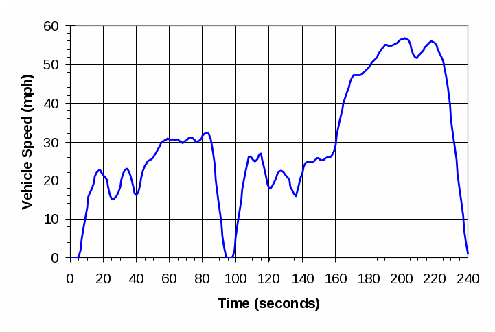
The index is analogous to a tailpipe emissions test based on the IM240 procedure, a variable-speed 240-second driving trace commonly used for tailpipe emissions testing in inspection and maintenance programs (Figure 1). Rather than attempt to estimate absolute IM240 emissions, we estimate the probability that a vehicle would “fail, ” i.e., would exceed a specified threshold level on the IM240, given its remote-sensing measurement(s). The threshold functions like a “cutpoint” in an actual I/M test, although the values to be used can be set specifically to meet the sampling objectives of this study.

Figure 1. Speed Trace for the IM240 test cycle.

The ”failure” probabilities are estimated using logistic regression on an applicable dataset, as shown in equations 1 and 2. Equation 1 shows the logit for the probability p_NOx that a vehicle’s NOx measurement on the IM240 would exceed some specified threshold h_NOx.

Equation 1

In this expression, f_NOx is the “fractile” of the vehicle’s NOx remote-sensing measurement, rather than the absolute measurement, taken to the 0.4^th power. The “fractile” is the “reverse-normalized rank” of the measurement, given by

Equation 2

where r_NOx is the rank of each measurement, assigned in reverse order, meaning that the highest measurement receives a rank of 1, and the smallest a rank of n, giving corresponding values of f_NOX of 1/n and 1.0, respectively. This non-parametric handling of the remote-sensing measurements is helpful in coping with two common aspects of remote-sensing data, namely, high variability and the presence of negative values. Because the remote sensing measurement represents pollutant concentration relative to CO₂ concentration within the exhaust plume, relative to background outside the plume, a high background value for whatever reason gives a negative remote-sensing value, i.e., the vehicle appears to be “cleaner than background.” Note also that the term β₀-β₁lnh acts as a constant intercept term for a given value of h.

Throughout we will illustrate the approach as developed for a sample of the general fleet in Denver, as described above. A set of cutpoints for each pollutant is shown in Table 2, and example coefficients for the logistic model in Table 3.

The fleet in the examples is broader than the target population for the study; it will be necessary to reparameterize the relationships for the target vehicle population before the onset of sampling.

Table 2. Example IM240 Cutpoints for Creation Replicate Modeling Datasets

Replicate	IM240 Cutpoint (g/mile)
Replicate	HC	CO	NOx
1	0.07	1.1	0.23
2	0.14	1.9	0.38
3	0.26	3.1	0.61
4	0.49	5.3	1.00
5	0.93	8.8	1.63
6	1.76	14.9	2.66

Table 3. Example Parameters for the Logistic Screening Model.

Parameter	HC	CO	NOx
β₀	2.8999	6.1709	4.0208
β₁	-6.6913	-4.9337	-6.1990
β₂	-1.6421	-2.0835	-2.1894

Figure 2. Fitted Values for NOx Remote-sensing and IM240 values.

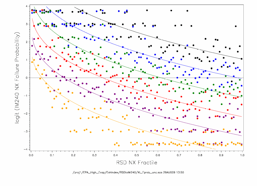
Figure 2 shows fitted values for NOx, for the six example thresholds shown in Table 2, with each threshold coded by color, as in Table 2. To illustrate an application of the logistic models we used a remote-sensing dataset collected over two days in the on-going Colorado fleet remote-sensing program. Figure 3 shows the model year distribution of the vehicles in the dataset, after filtering for valid remote-sensing and license plate values. As the target population includes most vehicles certified since 2004, the figure shows that the target population should currently include about 35% of vehicles in the light-duty fleet.

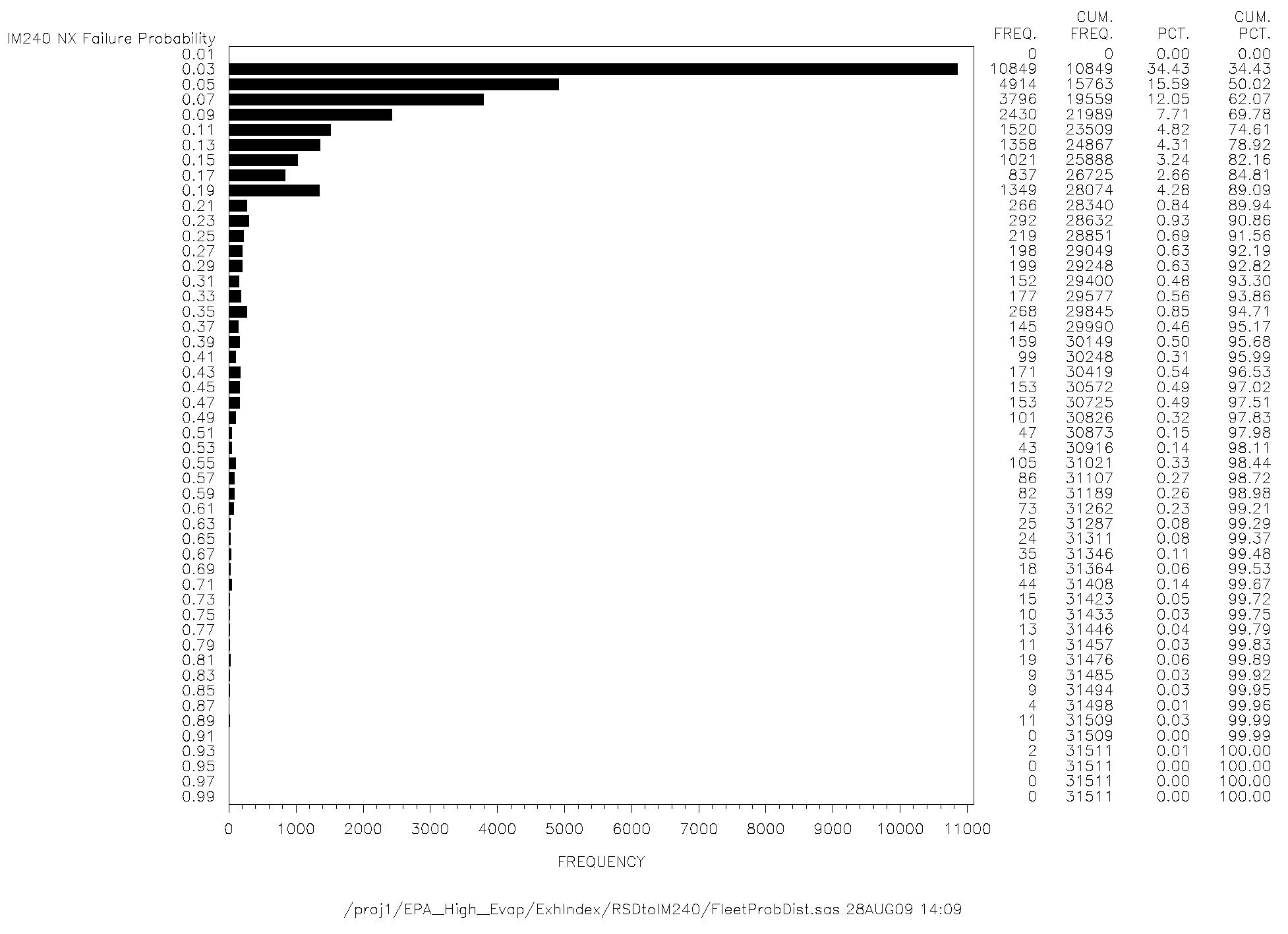
The models described above were applied to this dataset using IM240 cutpoints of 0.8, 15, and 2.0 g/mile for HC, CO, and NOx, respectively. In the discussion that follows we will focus on results for model years 2000-2010, as these more closely resemble the target population than vehicles in previous model years. The simulated distributions of IM240 failure probabilities for NOx are shown in Figure 4, which range from 0 to 63%.

Figure 3. Model-Year Distribution of the Application Dataset

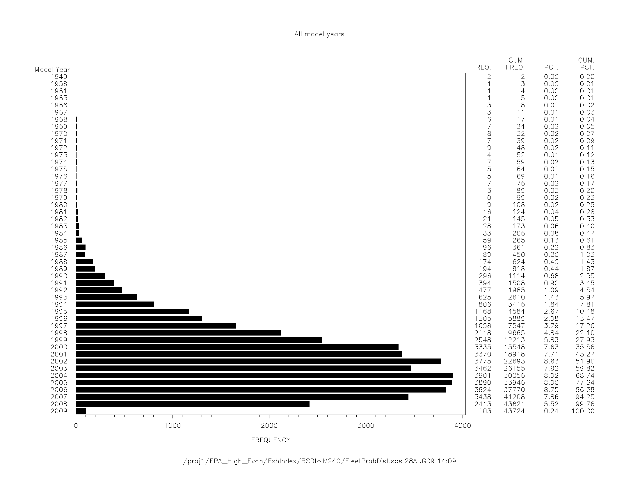
Figure 4. IM240 NOx Failure Probability Distribution for a 2.0 g/mile cutpoint (Model Years 2000-2010).

At this point, it is convenient to classify or “bin” the failure probabilities of the observations in the dataset. We created bins for each of the three pollutants and based on the logit of the failure probabilities predicted by the models. Table 4 shows the number of observations in each of the failure probability bins.

Table 4. Classification of Observations in the Application Dataset for Selected Cutpoints.

Bin Label	Range of IM240 Failure Probabilities	No. Observations
Bin Label	Range of IM240 Failure Probabilities	HC (0.8 g/mile)	CO (15.0 g/mile)	NOx (2.0 g/mile)
2	>82%	83	0	111
1	62 to 82%	145	5	515
0	38 to 62%	574	250	2,428
-1	18 to 38%	4,177	1,339	5,530
-2	8 to 18%	12,888	6,583	9,981
-3	3 to 8%	21,273	13,349	14,600
-4	<3%	0	17,614	5,975
	Total	39,140	39,140	39,140

At the conclusion of the preceding analysis, projected failure probabilities are available for all three pollutants. However, for sampling purposes it is highly desirable to resolve these results into a single variable. At the same time, sampling will be targeted to acquire roughly similar numbers of vehicles in each of the failure probability bins.

Because a vehicle with high emissions on one pollutant need not have high emissions on either of the other two (although such results are possible), sampling with respect to only one pollutant would give unsatisfactory results, with potentially distorted sampling distributions for the other two.

However, the failure probabilities for HC, CO, and NOx are somewhat correlated since there is a tendency for clean vehicles to have low emissions for all three, and the reverse for dirty vehicles. Consequently, principal components analysis can be used to generate a rotation of axes to create a new variable to serve as a single index incorporating all three pollutants. As with the fractiles, the index can then be classified as a convenient way to guide vehicle sampling. We have performed an example of this rotation of axes in the three dimensional logit space for the three pollutants. Using the observations in the application dataset, the first principal component PCA₁ is a linear combination of the HC, CO, and NOx logits:

Equation 3

Figure 5 shows the distribution of the first principal component values. As with the logits, it is convenient to classify the values of PCA₁ for sampling purposes, as shown in Table 5. Note that for high values of PCA₁, the IM240 failure probabilities of HC, CO, and NOx all tend to be high, and for low values of PCA₁, the IM240 failure probabilities of HC, CO, and NOx may tend to be correspondingly low.

A comparison of the counts of observations in the PCA₁ bins with respect to the IM240 failure probability bins shows for each pollutant a ridge of large counts that moves from high positive values to low (or negative values) This behaviour demonstrates that PCA₁ carries information about the IM240 failure probabilities for each of the three pollutants.

Figure 5. Distribution of First Principal Component Values (PCA1) based on IM240 cutpoints for HC, CO and NOx (0.8, 15, 2.0 g/mile).

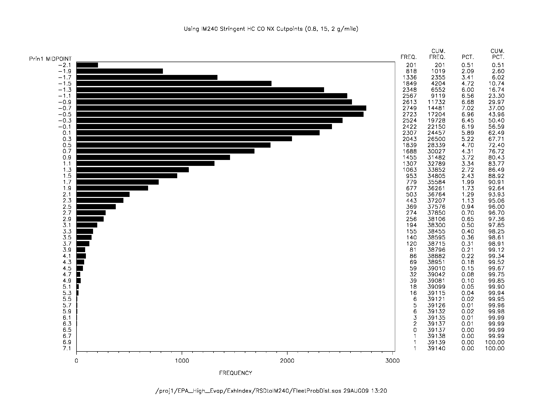
Table 5. Cross-tabulation of PCA₁ and Pollutant Failure Probability Bins for the Observation Dataset, by Pollutant.

		PCA₁ Bin
		6	5	4	3	2	1	-0	-1	-2	Total
Fprob HC Bin	2	13	22	19	17	12	0	0	0	0	83
	1	8	44	37	25	22	9	0	0	0	145
	0	0	63	180	135	115	73	8	0	0	574
	-1	0	10	211	785	1300	1170	659	42	0	4,177
	-2	0	0	5	157	1,480	3,899	4,925	2,422	0	12,888
	-3	0	0	0	3	131	1,753	5,996	10,182	3,208	21,273

Fprob CO Bin	1	1	2	2	0	0	60	0	0	0	5
	0	6	31	89	79	39	6	0	0	0	250
	-1	11	79	203	329	392	270	55	0	0	1,339
	-2	3	22	138	535	1,562	2,515	1,633	175	0	6,583
	-3	0	5	17	147	851	3,160	5,964	3,204	1	13,349
	-4	0	0	3	32	216	953	3,936	9,267	3,207	17,614

Fprob NOx Bin	2	5	16	29	23	24	14	0	0	0	111
	1	3	41	82	122	146	102	19	0	0	515
	0	10	34	142	384	743	817	298	0	0	2,428
	-1	3	37	148	360	1,081	2,007	1,612	282	0	5,530
	-2	0	11	42	179	779	2,376	4,127	2,466	1	9,981
	-3	0	0	8	44	231	1,237	4,318	7,114	1,648	14,600
	-4	0	0	1	10	56	351	1,214	2,784	1,559	5,975

Total		21	139	452	1,122	3,060	6,904	11,588	12,646	3,208	39,140

The pool of vehicles screened using remote sensing and having been assigned values of PCA₁, will serve as the sampling frame for the project.

2(b)(ii) Sample Size

For this collection we plan to recruit and measure emissions for approximately 250 vehicles. Assuming a response rate of about 30%, we plan to solicit approximately 830 vehicles.

The sample size will be based on two considerations: (1) the likelihood of capturing the “upper tail” or the high percentiles of the skewed emissions distribution, and (2), the power for a simple regression relating the the natural logarithm of the emission rate to vehicle age at time of measurement.

2(b)(ii)(1) Capturing high-emitting vehicles

With respect to this criterion, we have estimated sample size conservatively, to improve our ability to evaluate the screening index and to increase confidence that the sample would include high-emitting vehicles under the assumption that the screening index may not work efficiently.

Numbers of vehicles to be measured are given by an equation that relates the probability of capturing a specified population percentile (P) at a desired level of probability (K).^⁸ More specifically, the equation gives the probability K that at least one vehicle in the sample would be at or above the percentile level P (Equation 4).

Equation 4

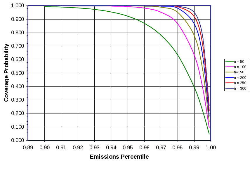
Figure 6 shows the coverage probability trends related to population percentile for selected sample sizes ranging from 50 to 300 vehicles. Based on these projections, the planned sample size (n = 250) should give virtual assurance that the 95th-percentile vehicle would be captured, and approximately 90% probability that the 99^th-percentile vehicle would be captured.

Note that these theoretical projections do not account for the possible effects of non-response bias which could reduce the prospects for capturing the dirtiest vehicles. Nor do they account for the effectiveness of screening, which should increase the likelihood of capturing high emitting vehicles, depending on its level of efficiency.

Figure 6. Estimated coverage probabilities for selected population percentiles, for a selection of sample sizes (Equation 4).

2(b)(ii)(2) Assessing age trends

An important analytic for this project is to estimate the trend (if any) in emissions versus vehicle age. This research question can be tested using a simple regression model of the natural log of NOx emissions vs. age.

Equation 5

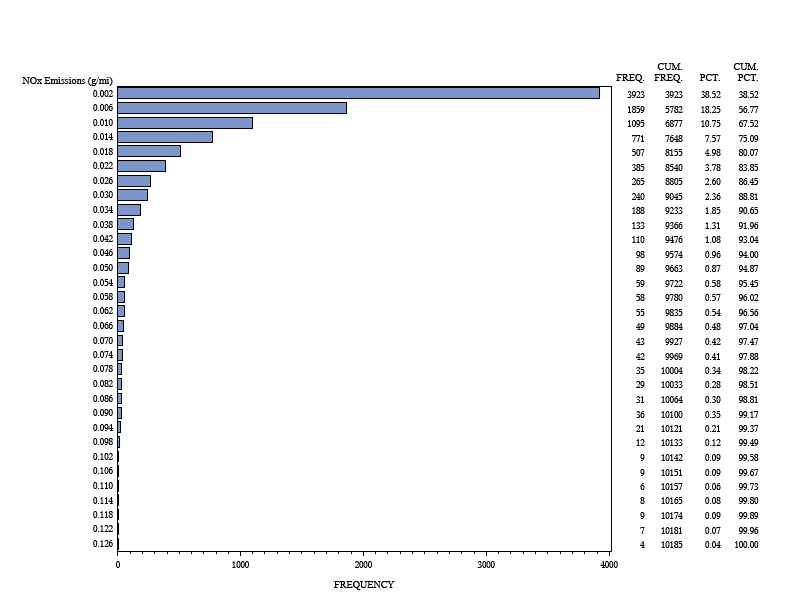
A simulation of this relationship for a population of N ~ 10,500 vehicles was performed using the parameters shown in Table 6. The emissions results represent the “hot-running” phase of the Federal Test Procedure, which is of interest because “hot-running” emissions are considerably more variable than start emissions (in relative terms), and thus represent the limiting factor in power estimation. The simulated population is shown in Figure 7 as lnNOx with respect to age, which shows a wide scatter around a definite age trend. Figure 8 shows NOx with respect to age, and illustrates the highly skewed nature of the distribution, and how the increase in the mean emissions level is driven by the “spreading” of the tail as vehicles age. Figure 9 shows a histogram of the log-normal population. Note that the population has been trimmed at the 97.5^th percentile level at each age to prevent simulation of unrealistically high values in the heavy log-normal upper tails. These figures highlight the relatively small numbers of vehicles in the tail that to be targeted by screening, as described above.

Table 6. Parameters describing a Simulated Population of lnNOx for Bin-5 Vehicles Between 0 and 6 Years of Age (N = 10,185 vehicles).

Source	DF	Sum-of-Squares	Mean Square	F-value	Pr > F
Model	1	457.76	457.76	267.63	<0.0001
Error	10,498	17,956.01	1.71
Total	10,499	18,413.77

	R²		Root MSE	Mean
	0.0249		1.307	-5.049

	Parameter	Estimate	Standard Error	t-value	Pr > \| t\|
	Intercept (b₀)	-5.411	0.02554	-2.1186	<0.0001
	Age (m)	0.1211	0.007400	16.36	<0.0001

Figure 7. Simulated lnNOx Emissions for a population of Bin-5 vehicles, represented by the Hot- Running Phase of the Federal Test Procedure. The red line represents the simulated age trend, reflecting an assumed slope of 0.12.

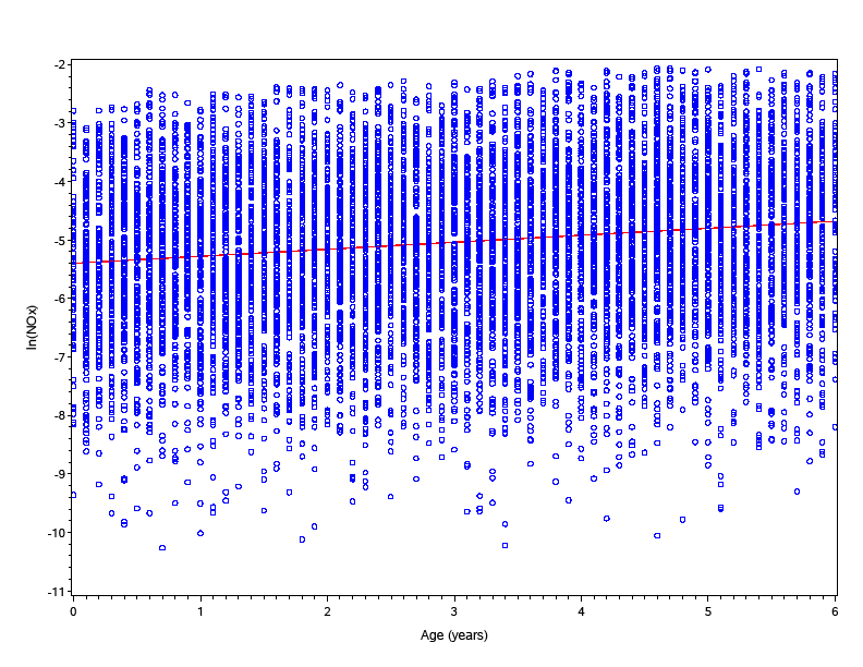
Figure 8. Simulated NOx Emissions for a population of Bin-5 vehicles, represented by the Hot- Running Phase of the Federal Test Procedure. The green and red lines represent the geometric and arithmetic means, respectively.

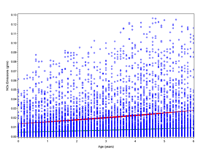
Figure 9. Histogram of Simulated NOx (reverse-transformed lnNOx) for a population of Bin-5 vehicles, represented by the Hot Running Phase of the Federal Test Procedure.

Needless to say, given the large “sample size,” the analysis of the simulated data in Table 6 above shows a highly significant effect for vehicle age. The overall F-test for goodness-of-fit as well as the parameter t-tests show very small p-values. It is important to note, however, the small R² of 0.022, which reflects the very high variability of measurements around the trend, which is characteristic of emissions data. The R² is the key parameter for purposes of power analysis for the prospective vehicle sample.

Table 7 shows estimated power levels for a Type-III F test for two confidence levels over a range of sample sizes. This analysis suggests that we might expect a power level for goodness-of-fit of approximately 60% at the 95% confidence level and 75% at the 90% confidence level.

Table 7. Projected Sample Sizes for a Range of Power Levels for an Analysis of lnNOx Emissions.

Table ?? Projected Sample Sizes for a Range of Power Levels For an analysis of lnNOx Emissions vs. Age. (Results for Type-III F test, R² = 0.02).
Power	Sample size (n) α = 0.05	Sample Size (n) α = 0.10
0.2	58	29
0.3	94	57
0.4	132	88
0.5	173	122
0.6	220	162
0.7	277	211
0.8	351	277
0.9	470	383

Table 8. Cross-tabulation of PCA1 and Failure Probability Bins for the Expected Vehicle Sample.

		PCA₁ Bin
		6	5	4	3	2	1	0	-1	-2	Total
Fprob HC Bin	2	4	7	3							14
	1	2	13	3	1						19
	0		19	27	5	2					53
	-1		3	28	21	16	5	1			74
	-2				6	19	10	9	4		48
	-3					1	5	14	13	9	42

Fprob CO Bin	1		1								1
	0	2	9	17	2						30
	-1	3	24	26	11	5					69
	-2	1	7	16	16	17	6	2			65
	-3		2	2	4	12	10	13	3		46
	-4			0	1	2	4	10	13	9	39

Fprob NOx Bin	2	2	5	5	1						13
	1	1	12	8	5	1		1			28
	0	3	10	19	12	9	2	1			56
	-1		11	21	11	14	7	6	1		72
	-2		3	7	4	10	6	7	2		39
	-3			1	1	3	2	8	7	5	27
	-4				1	1	1	3	5	4	15

Total		6	42	61	33	38	20	24	17	9	250

Note that through the use of screening index, the number of observations in each of the failure probability bins for the three pollutants is roughly similar. This can be put in perspective by comparing the counts in the Total column in the sample in Table 8 above with the corresponding counts in the Total column in the original dataset in Table 5. Please note that even though we have selected all vehicles in PCA₁ bins 5 and 6, the total number of vehicles in Bin 6 is not very large.

2(b)(ii)(3) Numbers of driving trips

As mentioned above, a “trip” is defined as a period of driving or operation that begins when a driver turns the engine on, and ends when the driver turns the engine off. As defined, the number of trips driven defines the number of engine starts, as each trip begins with a start.

For purposes of estimating emissions, we assume that the number of daily trips differs slightly between weekdays and weekends. For example, for passenger cars, we assume that average values are 5.89 and 5.30 trips per day for weekdays and weekends, respectively. To assess the expected behavior of the proposed sample, we have estimated the minimum detectable difference between weekdays and weekends with 95% power at the 5% confidence level.

The analysis is driven by the assumption that starts can be represented as a Poisson process, as described by the parameters in Table 9.

Table 9. Parameters for Simulated Poisson Counts of Trips over 8-week Measurement Period.

Parameter	Units	Weekday (1)	Weekend (2)	Difference (1) – (2)
Mean	Trips/day	5.89	5.71	0.18
Measurement period	Days	40	16
Trips per vehicle		235.60	91.36
Sample size	vehicles	250	250
Total trips	count	58,900	22,840
Test statistic (t)				3.98
Critical t				1.96
Confidence level				0.95
Power				0.95

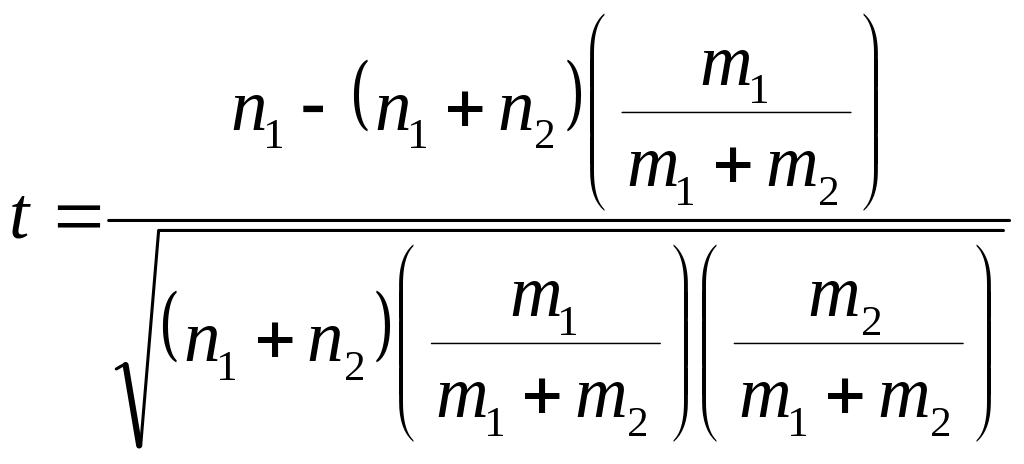
The weekday/weekend difference will be assessed by counting starts across all vehicles and days measured. Based on the counts, the test statistic t is estimated as

Equation 6

where n₁ and n₂ represent trip counts for weekdays and weekends, and m₁ and m₂ represent measurement periods for weekdays and weekends, respectively. For the proposed assumptions and sample size, a mean daily difference as small as 0.18 starts/vehicle/day would be detectable with 95% power and 95% confidence.

2(b)(iii) Stratification variables

In addition to screening, we plan to stratify the vehicles by age classes, as defined below in Table 10. This approach was adopted to avoid the potential for bias for selection of older vehicles over younger ones, were we to rank measurements and calculate fractiles across the entire six-year range.

Table 10. Age strata definitions for purposes of screening and sampling.

Age Range (years)	Class Midpoint (years)
0.0 <= age < 1.0	0.5
1.0 <= age < 2.0	1.5
2.0 <= age < 3.0	2.5
3.0 <= age < 4.0	3.5
4.0 <= age < 5.0	4.5
5.0 <= age <= 6.0	5.5

2(b)(iv) Sampling Method

The sampling method to be employed will be a form of “probability proportional to emissions”, as expressed through the PCA₁ screening index described above (see 2(b)(i) ). The sampling will be implemented through a process analogous to stratified sampling in which vehicles will be classified or “binned” by their PCA₁ values, and different sampling frequencies applied to each bin. The frequencies will range from sampling with certainty for the “dirtiest” vehicles to sampling fewer than 10 out of a 1,000 for the cleanest vehicles (Table 11).

Table 11. Sampling Fractions by Screening Index Bin (PCA1)

PCA₁ Bin	Sampling Fraction
6	1.0
5	1.0
4	0.50
3	0.10
2	0.040
1	0.010
0	0.007
-1	0.005
-2	0.008

2(b)(v) Multi-Stage Sampling

This collection will not employ multi-stage sampling.

2(c) Precision Requirements

2(c)(i) Precision Targets

Precision targets are geared to the power analyses performed for estimation of sample size, as described above.

For purposes of capturing emissions from vehicles in the high percentiles of the distribution, our targets are to achieve 99% and 95% confidence levels that the 95^th and 99^th percentiles have been captured, respectively.

For purposes of estimating the age trend of lnNOx, the precision target is a 90% confidence level for the type III F test of fit at the 75% power level.

For purposes of estimating numbers of starts for weekdays and weekends, the precision target is 95% power at 95% confidence for a difference between Poisson counts of driving trips.

2(c)(ii) Non-Sampling Error

2(c)(ii)(1) Frame-coverage error

This error is defined as potential bias in key variables resulting from imperfections in the sample frame. The central issue is incomplete coverage, in which members of the target population are simply absent from the frame. The bias that may result from incomplete coverage may reduce the representativeness of the sample in a way analogous to that from whole-survey non-response. In this project, because the sample frame will be constructed from the pool of vehicles measured by remote sensing for screening purposes, actual frame coverage may be limited by factors that reduce representative coverage of the entire light-duty fleet. One such factor may be the the inability to obtain valid license plate readings on some fraction of measured vehicles. To minimize this factor, we plan to have license plates read manually, which gives a higher yield rate than the use of software. In any case, given that the frame will be based on vehicles themselves, rather than households, it will be possible to address frame coverage issues by post-stratification against the state vehicle registration database.

2(c)(ii)(2) Non-response error

As in any survey, non-response is one of the most important potential sources of error in final results. Survey non-response occurs when no response at all is obtained from a potential participant in the study, whereas item-nonresponse occurs when a respondent provides responses to some but not all items. Survey non-response occurs if a respondent refuses to participate. Item-nonresponse may occur in a number of ways. A respondent may answer some items but refuse others, or may break off an interview for unrelated reasons. A form of item-nonresponse detrimental to emissions measurement but unrelated to the respondent could occur in cases where equipment malfunction or measurement errors make emissions datasets unsuitable for subsequent analysis.

2(c)(ii)(3) Measurement error

The measurement of exhaust emissions involves the use of complex instrumentation in a non-laboratory environment. The potential for measurement error in the RSD equipment and PEMS equipment is well understood. During field work, all instruments, including the remote sensor and PEMS equipment will be calibrated regularly following standard operating procedures.

2(c)(ii)(4) Equipment malfunction

Following the measurements based on the various instruments, quality-assurance measures will be undertaken to verify that the instruments operated correctly and that the results are reliable for further analysis. The QA process will involve the use of computer programs that automatically scan the time-series for patterns that may suggest instrument error, combined with graphic presentation of the data to allow case-by-case visual inspection.

2(c)(ii)(5) Respondent error

The emphasis on collection of key information for the survey through direct inspection and instrumentation involves a conscious decision to reduce reliance on human memory to the maximum extent possible. A primary example is the use of electronic dataloggers to measure vehicle emissions and activity. As much as possible, we have restricted interview items to general questions that can be easily answered without involved or detailed estimation and without heavy reliance on human memory.

2(c)(ii)(6) Data entry error

Emissions results and other data collected electronically will not be input manually. Data files will be downloaded directly from the measurement instrument and transferred to the database, following quality-assurance procedures.

2(d) Questionnaire

During the initial phone contact, we will conduct a very brief interview to verify that the respondent owns the vehicle selected, to solicit participation, and to schedule an appointment to bring their vehicle to the test facility. This script is presented as Appendix A.

Vehicle owners that participate in the study will receive another brief interview when they arrive at the testing facility. We will collect recent vehicle usage and maintenance history information using the questionnaire in Appendix B. The questionnaire contains ten items designed to assess general maintenance history of the vehicle, including major repairs or accidents.

Before instrumentation, an additional twelve items of information will be collected from the vehicle itself by inspection, as shown in Appendix C. These items are redundant with information in the sample frame, but redundant collection at the time of measurement will allow confirmation of the vehicle’s identity as well as verification of the sample frame. Additionally, technicians will take several photographs to document key information on the vehicle.

3.0 Pretests and Pilot Tests

The sampling and recruitment methods to be used in this collection will be similar to those used in other studies that we have undertaken within the past two years (control number 2060-0615). The recruitment approach and logistics will be similar enough to those used for the previous collection that the current collection will employ approaches that have been tried in the field.

4.0 Collection Methods and Follow-Up

Implementation of the program will include the following elements:

4(a) Screening Methods

Remote sensing vans will be deployed throughout the Detroit Metropolitan area to collect screening measurements on the vehicle population. Sites will be selected to be representative of the population and appropriate for the remote-sensing technique. Criteria for a good site include moderate vehicle speed, moderate acceleration, mild positive slope, a single lane of traffic, a safe area to park the van and deploy instruments, and a moderate level of vehicle traffic.

All vehicles will have the emissions plume scanned by an RSD instrument to measure emissions concentrations. The instruments perform these measurements by shining a light beam across the roadway to a receptor. Associated equipment will also simultaneously determine other quantities. These measurements are collected without without imposing any burden on vehicle owners. For each vehicle the following quantities will automatically be taken as the vehicle drive past the RSD instrument:

Item 1: DateTime: The date, hour, minute, and second of the RSD measurement.
Item 2: Speed and Acceleration: The speed and acceleration of the vehicle.
Item 3: Emissions Absorbances: The absorbances (concentration × pathlength) of HC, CO, NO, and CO₂ in the vehicle’s plume.
Item 4: License Plate: A digital image of the rear of the vehicle so that the license plate may be read.

4(b) Solicitation Methods

Based on the screening level and associated sampling frequency, a sample of passenger cars and light-duty trucks will be selected for solicitation. The sample will be released in a series of replicates, each of which will be thoroughly processed before subsequent replicates are released.

Step 1: Selected vehicles will be transmitted to the call center for solicitation.

Step 2: Vehicle owners will be sent an initial notification of the study by mail.

Step 3: Potential respondents having received the mailing will be contacted by phone. Interviewers will make multiple attempts at contact with each respondent. During the phone contact the interviewer will notify potential respondents that they will receive a $10 incentive whether or not they participate.

Step 4: During initial or successive phone contacts interviewers will attempt to schedule an appointment for the respondent to bring their vehicle to the project facility for measurement.

Step 5: Upon arrival for an appointment at the test facility, the respondent will participate in the vehicle survey (Appendix B). The brief interview will obtain information regarding recent maintenance, malfunctions, service needed, etc. An overall assessment will be made of the vehicle’s interior and exterior condition, which will be reviewed with and signed by the vehicle’s driver. After these steps, technical personnel will install instrumentation and perform measurement procedures on the vehicle. At the respondent’s option, rental vehicles will be available for their use while their own vehicle is being measured. Following completion of measurement, technicians will remove the instrumentation and return the vehicle to the respondent. The respondent will be provided an additional incentive at the completion of their participation.

4(c) Measurement Methods

After receiving final consent to instrument the vehicle, technical personnel will perform the following steps:

Step 6: Collect Vehicle information – A technician will visually examine the vehicle to collect the vehicle identity information listed in Appendix C. Some items will be documented with a camera to reduce the chance of transcription errors.

Step 7: Each vehicle will receive a unique identification code for documentation and tracking purposes, and will then be inspected for measurement feasibility. This preliminary inspection will involve a short road test to check the vehicle’s brakes and steering. A brief check will also be made of the vehicle’s exhaust system to ensure that no major leaks are present (which could affect emissions measurements). A fluid check will be performed to reduce the possibility of overheating, low oil operation, or other problems during instrumentation or measurement.

Step 8: If the vehicle is not considered safe for instrumentation, it will be returned to the respondent, whose participation would then be complete. If the vehicle is considered safe for instrumentation technicians will install a portable emissions measurement system. They will then perform warm-up and check procedures to verify correct functioning of the various systems and analyzers. As necessary, systems will be audited and recalibrated to ensure accuracy.

A test driver will then start the vehicle and take it over a pre-arranged route designed to include selected driving patterns including stop-and-go traffic, acceleration at high speed, freeway driving and idling. Following completion of the first route, the vehicle will be parked for a specified period with the engine off, after which the engine will be re-started and the driving route repeated. Repetition of the route allows for replication as well as capture of the start emissions increment. At the completion of the drive routes, the vehicle will be parked overnight with the instrumentation installed.

Step 9: The following morning, the instrumentation will be turned on and warmed up as before. When the system is ready the test driver will restart the car, with the engine cold, and repeat the drive route. After completion of the first route, the car will be again parked with the engine off and the route repeated.

Step 10: Following completion of the final driving route, technicians will download and backup the emissons datafile. They will perform designated post-check procedures and remove the emissions instrumentation from the vehicle.

Step 11: Technicians will install a “portable activity measurement system” (PAMS) on the vehicle. The PAMS will record selected operating parameters while the vehicle is operating that will allow characterization of trips and other driving patterns.

Step 12: The vehicle will be returned to the respondent. The respondent will drive the vehicle for a specified measurement period of three months with the PAMS installed.

Step 13: At the completion of the measurement period, technicians will retrieve the PAMS unit. At the respondents’ convenience, a field team will travel to the respondents’ locations to spare the respondent the additional burden of returning to the facility for instrument removal.

5.0 Analyzing and Reporting Survey Results

5(a) Data Preparation

5(a)(i) Interview Information

During field work interviewers will record respondent’s information on paper questionnaires and interview sheets. At the end of each day, personnel will scan the field copies into computer files to prevent loss of data should the originals be lost or damaged. Computer files will be backed up and stored in different locations.

Personnel trained in data entry will enter the survey information into electronic data files. In this process, we plan to use “double-entry” techniques, meaning that all information will be keyed in independently by two individuals. Following an item-by-item comparison of the two versions, all instances where the files differ will be manually checked to ensure accuracy.

5(a)(ii) Emissions Data

Technicians will download emissions and activity data directly from the instruments prior to removal. Following calibration and quality assurance, these data will be compiled into relational-database format, linking emissions data to relevant vehicle and engine information. During the loading process, additional quality-assurance measures will be taken to ensure that the instrumentation was operating correctly and that the data are reliable for further analysis.

5(b) Data Analysis

Using the simulated population of NOx emissions developed for purposes of sample-size analysis, we have simulated a process of sampling and analysis, including the following steps:

1) Sampling the population

2) Simulating non-response

3) Analyzing the data for age trend

4) Using the screening measure to investigate non-response bias

5(b)(i) Sampling the population

“Sampling the population” involved simulating the steps of remote-sensing, development of the screening index, and assignment of sampling weights.

The simulated “remote-sensing measurements” were designed as non-negative values showing broad correlation to the “actual” emission values. This translation was achieved simply by adding an additional normally-distributed disturbance in ln-space and applying a positive offset such that most of the simulated values would be positive. A given remote-sensing measurement RSD_i was generated by exponentiating the sum of a randomly generated lnNOx measurement u, a random normal variate distributed with mean 0.0 and standard deviation σ_RSDZ, and a positive offset of 9.0. The value of σ_RSDwas set at 1.2; Z represents a standard normal variate.

Equation 7

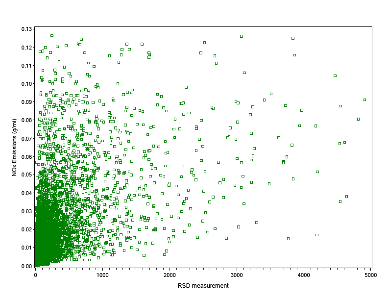
The resulting estimates pictured in Figure 10 show a realistic degree of spread and scatter. While the parametric or Pearson correlation for these variates is low (~0.45), the corresponding non-parametric Spearman correlation is reasonably high (~0.77).

Figure 10. Simulated “RSD measurements” in relation to corresponding “emissions measurements” for the simulated Bin-5 vehicle population.

Having “performed remote-sensing,” the next step was to simulate the development of the screening index. For this exercise, we simulated screening in terms of a single pollutant, NOx, but did not attempt to model the correlation among pollutants or the principal components analysis previously described.

The logit for exceedance of the target threshold was calculated using Equation 1, having calculated “fractiles” as in Equation 2, and using the parameters listed in Table 12. These parameters are similar to those in Table 1, but modified to apply to the target population. The assigned cutpoint (h=0.05 g/mile) was assigned based on actual Bin-5 results and correponds to approximately the 95^th percentile at age 1. Ranking and calculation of ‘fractiles’ (f) was performed separately within six age strata, as defined above in 2(b)(iii).

Table 12. Parameters to estimate simulated logits for the probability that simulated NOx would exceed the cutpoint of 0.05 g/mile.

parameter	Estimate
β₀	-3.0
β₁	-6.2
β₂	-2.1
h	0.05

As mentioned, for this exercise the logit for NOx was used as the screening index. Accordingly, we binned it for sampling purposes, as shown in Table 13 (Note that the Bins in Table13, based on the simulation, are not the same as those in Table 11, which as based on actual data). The structure of the simulated vehicle population, by screening Bin and age strata, is shown in Table 10. The uniformity of the population profile across screening bins within age classes reflects the calculation of fractiles based on ranks, rather than on absolute remote sensing values.

Table 13. Simulated Classes (“Bins”) for the NOx-based Screening Index

Lower bound	Upper bound	Midpoint	Bin Label
	-3.00	-3.300	0
-3.00	-2.15	-2.575	1
-2.15	-1.30	-1.725	2
-1.30	-0.45	-0.875	3
-0.45	0.40	-0.025	4
0.40	1.25	0.825	5
1.25	2.10	1.675	6
2.10	3.00	2.525	7
3.00		3.375	8

Table 14. Structure of simulated Population, by Screening Bin and Age class.

Bin	Age Stratum (Midpoint, years)
	0.5	1.5	2.5	3.5	4.5	5.5	Total
1	451	471	477	478	475	487	2,839
2	404	422	427	428	426	436	2,543
3	306	319	324	324	322	330	1,925
4	217	227	229	231	229	235	1,368
5	140	145	148	148	147	151	879
6	74	78	79	79	79	80	469
7	26	27	27	27	27	28	162
Total	1,618	1,689	1,711	1,715	1,705	1,747	10,185

To simulate analysis, we drew “samples” from the simulated population. The overall sample was targeted to the same size as that described previously (n_total~830). For purposes of illustration, the characteristics of one replicate sample are shown in Table 15. Within each of the 42 screening-bin × age-Class cells, a sampling rate was assigned so as to achieve a “sub-sample” of approximately 20 vehicles, accordingly, the sampling frequency in each bin was calculated as 20/n. As expected, the sampling process achieved broadly uniform sub-samples in each cell, in contrast to the pronounced pyramidal shape of the population.

Table 15. Structure of a Sample of the Simulated Population, by Screening Bin and Age Class

Bin	Age Stratum (Midpoint, years)
	0.5	1.5	2.5	3.5	4.5	5.5	Total
1	17	23	22	18	18	19	117
2	21	27	19	15	20	22	124
3	20	23	13	25	16	19	116
4	17	20	17	21	23	17	115
5	12	19	32	17	19	17	116
6	20	22	17	23	26	20	128
7	20	16	13	17	16	15	97
Total	127	150	133	136	138	129	813

5(b)(ii) Simulating Response

A first step in analysis of response will be to assess response patterns in relation to characteristics of respondents or their vehicles. Detailed demographic data on vehicle owners, such as household size, age, educational level or income will not be available. However, vehicle characteristics such as number of vehicles owned, model year, vehicle type, and vehicle manufacturer will be readily available. Additional items may be constructed to incorporate information such as maintenance level and occurrence of accidents. As an index of burden, it will also be possible to construct additional measures such as driving distances from the respondents’ home addresses to the study site. Based on these characteristics, response patterns can be assessed through response cells or logistic regression. This level of analysis may identify patterns of interest, may suggest potential for non-response bias, and serve as the basis for non-response weighting, but is not sufficient to confirm or estimate bias. An advantage of having screened all vehicles in the sample frame is that it may be possible to assess response patterns using the screening measure as an index of exhaust emissions, the response variable for the study. The success of this analysis will depend on the degree of correlation between the screening measure (RSD emissions) and the “truth” measurement (PEMS emissions). If this correlation is fairly high to high it should be possible to relate participation directly to emissions.

For the sample, we simulated participant response as an additional “sampling process.” We projected a worst case in which response was inversely related to vehicle emissions. However, in contrast to the sampling, the response process was related to the “actual” emissions measurement, rather than the remote-sensing screening measurement. This approach reflects a worst-case assumption that vehicle owners are to some degree aware of their emissions and that owners of “dirty” vehicles respond at lower rates than those of “clean” vehicles.

To implement this approach, we ranked all measurements in the sample by their “actual” values and assigned them to quintile groups. We assigned each quintile a response rate, designed to give an overall response rate of about 30%, which we believe to be achievable, and which would give measurement samples of about 250 vehicles.

Table 16. Assigned Response Rates for the Replicate Samples

Quintile	Percentile Range	Response Rate
5	80 - 100	0.10
4	60 - 80	0.18
3	40 - 60	0.36
2	20 - 40	0.40
1	0 - 20	0.43

Using these response rates, a sub-sample of respondents was drawn from the initial sample. We re-classified respondents and non-respondents by the seven screening bins and re-calculated effective response rates for each bin. The secondary respondent sample and corresponding response rates are portrayed in Table 17 and Table 18, respectively.

Table 17. Structure of a Secondary “Respondent” Sample, by Screening Bin and Age Class.

Bin	Age Stratum (Midpoint, years)
	0.5	1.5	2.5	3.5	4.5	5.5	Total
1	3	12	11	3	7	7	43
2	5	9	9	8	8	11	50
3	3	12	6	6	4	10	41
4	7	6	6	6	9	5	39
5	3	4	12	3	6	6	34
6	5	3	3		4	5	20
7	2	3	5	1	2	1	14
Total	28	49	52	27	40	45	241

Table 18. Simulated Response Rates for a Vehicle Sample, by Screening Bin and Age Class.

Bin	Age Stratum (midpoint, years)
	0.5	1.5	2.5	3.5	4.5	5.5
1	0.17	0.52	0.50	0.17	0.39	0.37
2	0.24	0.33	0.47	0.53	0.40	0.50
3	0.15	0.52	0.46	0.24	0.25	0.53
4	0.41	0.30	0.35	0.29	0.39	0.29
5	0.25	0.21	0.38	0.18	0.32	0.35
6	0.25	0.14	0.18	0.00	0.13	0.07
7	0.10	0.19	0.38	0.06	0.13	0.07

As shown in Table 15, the sample is designed to be “top heavy” with respect to the screening index, to ensure representation of the high-emitting vehicles. Having employed this sample design, however, the using of sample weighting in analysis is critical. Thus, using sampling frequencies (f_sample) and response rates (f_resp), we calculated final weights as the product of their reciprocals.

Equation 8

Table 19 shows sums of final weights for the respondent sample. The weights recreate the pyramidal shape of the vehicle population, as expected. However, the sum of the sampling weights falls slightly short of the population total, reflecting nonresponse in cells where no respondents “participated”, which cannot be compensated by non-response weighting.

Table 19. Sums of Final Weights for the Respondent Sample, by Screening Bin and Age Class.

Bin	Age Stratum (Midpoint, years)
	0.5	1.5	2.5	3.5	4.5	5.5	Total
1	451	471	477	478	475	487	2,839
2	404	422	427	428	426	436	2,543
3	306	319	324	324	322	330	1,925
4	217	227	229	231	229	235	1,368
5	140	145	148	148	147	151	879
6	74	78	79		79	80	390
7	26	27	27	27	27	28	162
Total	1,618	1,689	1,711	1,636	1,705	1,747	10,106

5(b)(iii) Analyzing for Age Trend

Having calculated final weights based on sampling and non-response weights, it is possible to analyze the simulated vehicle samples for age trend. This step estimates the “actual” population values (Table 6), based on the samples, using a simple model for age (Equation 5).

Table 20. Simulated Goodness-of-Fit and Model Parameters for Models of lnNOx v. Age for two Replicate Samples.

Sample	Parameter	Estimate	Std. Error	t	P>t
1 (R²= 0.024)	Intercept	-5.358	0.113	-47.29	<0.000001
(repl 7)	Slope	0.1671	0.0348	4.79	0.000002
2 (R²= 0.0032)	Intercept	-5.076	0.157	-32.41	<0.000001
(repl 2)	Slope	0.01739	0.0428	0.406	0.68

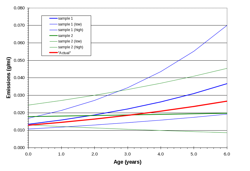
Figure 11 represents the mean trend predicted from the sample, as well as the upper and lower 95% confidence bounds. The bounds were calculated using the upper and lower confidence limits of intercepts and slopes, respectively. They assume no correlation between intercepts and slopes for specific samples and may thus be wider than expected in real data. In both cases, the confidence bounds capture the actual values.

In the second sample the slope term is not significant, whereas in the first it is highly significant. This result is consistent with the results of the power analysis, which suggested that the chances of Type-II error would be in the range of 30-40%. At first glance it is difficult to tell whether the error is due to non-response, or to sampling error as such.

Figure 11. Simulated Age Trends for the Population (“Actual”) and two Samples.

5(b)(iv) Investigating Non-response Bias

Due in large measure to the difficulty and expense of measurement, which increases the challenge of obtaining high levels of response, the possibility that non-response may reduce the accuracy of emissions estimates is a long-standing concern. Anecdotal evidence suggests that some motorists with high emissions are aware of the fact, and presumably avoid participation in studies. Presumably, this generalization is more applicable in areas with Inspection-and-Maintenance programs than in those without.

In previous efforts, we have attempted to address the question by comparing the demographics or geographic dispersion of respondents and non-respondents, and by comparing results for respondents and converted refusals. While failure to see marked or significant differences between respondents and non-respondents with respect to these characteristics may suggest that non-response does not substantially affect the results, these analyses cannot definitively rule out the possibility of non-response bias.

An advantage with the current project is that the construction of the sampling pool using the remote-sensing screening measure gives at least a rough index of emissions for all vehicles in the sampling frame, including respondents and non-respondents. Our goal is to investigate the prospects for making use of the screening index to identify and characterize non-response bias. As with the sampling process, the efficiency of the index for this analysis will depend on the degree of correlation between screening and actual measurements.

A simple initial approach would be to average the remote-sensing measurements for the population and for the sample (using final weights), by screening bin and age class. Again, we have calculated these values using the simulated “remote-sensing” values, which have an overall Spearman rank correlation of 0.77 with the “actual” values.

Figure 12. Mean Simulated Remote-Sensing Values for the Population and for the Sample (Replicate 1), by Screening Bin and Age Class. (a) All values. (b) Close-up view of values < 1,000.

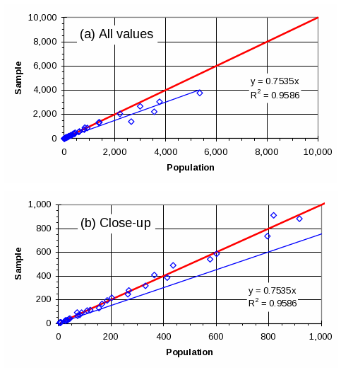
Figure 13. Mean Simulated Remote-Sensing Values for the Population and for the Sample (Replicate 2), by Screening Bin and Age Class. (a) All values. (b) Close-up view of values < 1,000.

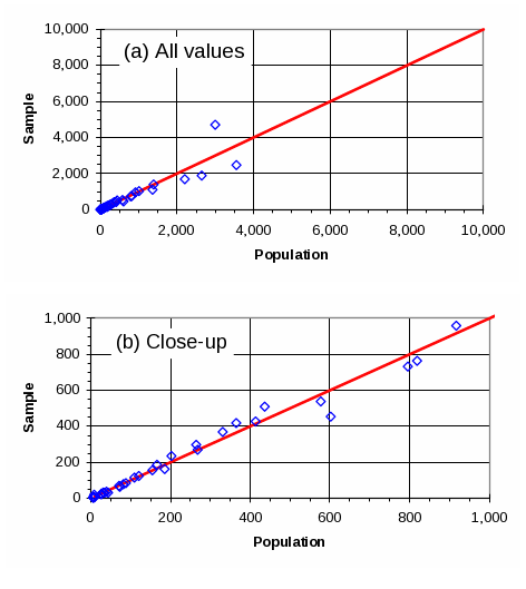
These results appear consistent with the occurrence of non-response bias, in that agreement falls off as the response rate declines (Table 18). However, if this were the case, it is important to note that the effects differ in the two replicates, with replicates 1 and 2 showing positive and negative biases for the slope terms, respectively (Table 20, Figure 11).

A tentative conclusion from this exercise is that, in practice, the effects of non-response bias may be difficult to distinguish from sampling error. Stated differently, it appears that the presence of non-response bias may affect inferences drawn from samples by compounding sampling error, with results that are difficult to predict. It is important to further test these conclusions, drawn from simulations, with actual screening and emissions data.

5(c) Reporting Results

Results of the study will be made available to the public and within the agency through the following means:

Results of the study will be uploaded into the Mobile Source Observation Database (MSOD). This database contains emissions measurements and supporting data, develop dand maintained by the USEPA National Vehicle & Fuel Emissions Laboratory. Results for key variables pluse necessary metadata will be entered. However, the identities of respondents will be protected. Specific identifying information will not be entered. This database is available to the public, upon request.

Appendix A: Telephone Script

INTRO:

Hello, my name is __________________, and I’m calling on behalf of the U.S. Environmental Protection Agency. May I speak with ___________________?

I’m following up on the letter we mailed you regarding the study of passenger vehicle emissions. Did you receive and read our letter?

YES

Great. As a reminder, the EPA is conducting a study of passenger vehicle emissions and is looking for qualified participants. In order for you to qualify for this study I need to collect some basic information about your vehicle. Within the next few weeks you will receive $10 for talking to me today.

We are inviting people who live in the [greater] Detroit area like yourself to take part in a study of vehicle emissions. The main goal of the research is to study tailpipe emissions from some vehicles manufactured since 2004. As I mentioned, we will be sending you $10 with our thanks just for talking to us.

You may be asked to set up and appointment with a team of specially trained professional engineers. You would bring your vehicle to our test facility, where the engineers will install instruments on your vehicle to measure its emissions. Then a trained driver will drive the vehicle over a route like the driving you might do each day. We’ll keep your vehicle overnight, and repeat the emissions measurements the next morning.

After that, technicians will remove the emissions instruments and install a small instrument that will measure certain operating parameters of your car while you drive normally over the next [MEASUREMENT PERIOD] weeks. The instrument is very small and will not interfere with your driving or use of the vehicle. We will then release the vehicle to you and provide you with an inventive of [INCENTIVE] to reimburse you for your inconvenience and expense.

This information will allow us to relate the emissions that we measure to how people actually drive. For example, it will enable us to understand how often, and how far people drive, as well as how they speed up, slow down and brake. These aspects of driver behavior are important to understanding emissions, because the way vehicles emit depends heavily on how they are driven.

After the completion of the [MEASUREMENT PERIOD], our technicians will be happy to come to you to disinstall the instrument. At that time, we will provide you with a final incentive of [INCENTIVE].

We are happy to accommodate your preference for dates to come in and can work around your schedule. This study is for scientific research purposes so that all information about you will be kept confidential.

To see if you qualify I would like to obtain some information about your household and vehicles.

Q1:

My records show that you live in [AREA]. Is that correct?

YES

OTHER/SPECIFY

REFUSED

Q2:

Our records show that you drive a [COLOR]-colored [MAKE] [MODEL]. Is this correct?

YES

OTHER/SPECIFY

REFUSED

EXPL:

Based on the information you’ve provided us, you are eligible to participate. We would like to schedule you for an appointment.

Q3:

When would you like to schedule an appointment?

NOW

LATER

OTHER/SPECIFY

REFUSED

ASSN:

We have an opening on [DATE]. Would you be able to bring your vehicle to our facility at

[ADDRESS], [CITY]?

IF NO: what day/date would work best for you?

[LIST DATES]:

REFUSED

TSLOT:

We have the following time slots available. Which would you prefer?

[LIST TIMES]:

REFUSED

CPHON:

Is [PHONE] the best number to reach you?

YES

IF NO: Is there another number where we can reach you?

TEL02:

___ ___ ___ - ___ ___ ___ - ___ ___ ___ ___.

THANK:

Great. So to confirm, your appointment is scheduled for [DATE], at [TIME]. We will shortly mail you a letter with $10, a reminder of your day and time, and contact information in case you have any questions. Thank you so much for your help and participation in this very important study!

Appendix B: Questionnaire

Measurement Questionnaire

Respondent ID	__ __ __ __ __ __ __ __ __ __ __ __ __ __ __ __ __ __ __ __ __ __ __
Vehicle ID	__ __ __ __ __ __ __ __ __ __ __ __ __ __ __ __ __ __ __ __ __ __ __
Interviewer ID	__ __ __ __ __ __ __ __ __ __ __ __ __ __ __ __ __ __ __ __ __ __ __
Date (mm/dd/yyyy)	__ __ / __ __ / __ __ __ __.

GREETING:

Hello, I am <NAME>, with <CONTRACTOR>. You completed a phone conversation with us on <DATE>. At that time, you consented to allow us to place an instrument on your vehicle to measure its emissions. At that time, we made an appointment for this visit.

We want to emphasize that the instrument is noninstrusive. It will not interfere with your vehicle or with your driving in any way. Technicians will install the equipment, after which one of our drivers will drive the vehicle over a carefully designed drive route to measure its emissions during different kinds of driving, such as residential streets, thoroughfares, and the freeway.

We’ll keep your vehicle overnight, and repeat the emissions measurements tomorrow morning.

We will then release the vehicle to you and provide you with an inventive of [INCENTIVE] to reimburse you for your inconvenience and expense.

After the completion of the [MEASUREMENT PERIOD], our technicians will be happy to come to you to disinstall the instrument. At that time, we will provide you with a final incentive of [INCENTIVE], and your participation in the study will be complete.

Your participation is entirely voluntary, and your name will not be connected with the data in any way.

We estimate that this process will take approximately [duration] hours.

Do you have any questions? May we proceed?

ANSWER QUESTIONS, PROCEED IF R CONSENTS.

ENTER TIME NOW: __ __ : __ __.

Q1. How long have you owned the vehicle: __ __ years.

REFUSED 999.

Q2. Do you park the car in a garage at night?

YES 1

NO 0

DON’T KNOW 998

REFUSED 999

Q3 As far as you know, has the vehicle been in any accidents?

YES 1

NO 0

DON’T KNOW 998

REFUSED 999

IF YES, DESCRIBE ____________________________________________________

___________________________________________________________________________.

Q4. Can you remember when the oil was last changed in this vehicle?

YES 1

NO 0

DON’T KNOW 998

REFUSED 999

IF YES, ENTER DATE: month: __ __ year: __ __ __ __, AND GO TO Q3,

IF NO, GO TO Q2

Q5 Can you tell me which answer is closest to when you think the oil was last changed?

DURING THE LAST MONTH 1

DURING THE LAST 2 TO 3 MONTHS 2

DURING THE LAST 3 TO 6 MONTHS 3

DURING THE LAST 6 TO 12 MONTHS 4

MORE THAN 12 MONTHS 5

DON’T KNOW 998

REFUSED 999

Q6 Have you had the muffler replaced?

YES 1

NO 0

DON’T KNOW 998

REFUSED 999

IF YES, GO TO Q4,

IF NO, GO TO Q5.

Q7 Can you tell me which answer is closet to when the muffler was replaced?

DURING THE LAST MONTH 1

DURING THE LAST 2 TO 3 MONTHS 2

DURING THE LAST 3 TO 6 MONTHS 3

DURING THE LAST 6 TO 12 MONTHS 4

MORE THAN 12 MONTHS 5

DON’T KNOW 998

REFUSED 999

Q8 Have you had the catalytic converter replaced?

(explain, if necessary, that in some vehicles the exhaust system, including the catalyst, manifold, muffler and tailpipe may be a single unit, and must be replaced as such, and in others, a modular system may allow these parts to be replaced individually).

YES 1

NO 0

DON’T KNOW 998

REFUSED 999

IF YES, GO TO Q4,

IF NO, GO TO Q5.

Q9 Can you tell me which answer is closet to when the catalyst was replaced?

DURING THE LAST MONTH 1

DURING THE LAST 2 TO 3 MONTHS 2

DURING THE LAST 3 TO 6 MONTHS 3

DURING THE LAST 6 TO 12 MONTHS 4

MORE THAN 12 MONTHS 5

DON’T KNOW 998

REFUSED 999

Q10 Have you had other major repair or maintenance performed on the vehicle within the last 12 months?

YES 1

NO 0

DON’T KNOW 998

REFUSED 999

IF YES, DESCRIBE ____________________________________________________

_____________________________________________________________________.

EXIT: Thank you. Those are all the questions I have. We appreciate your taking time to help with the research project.

Appendix C: Vehicle Information

Respondent ID	__ __ __ __ __ __ __ __ __ __ __ __ __ __ __ __ __ __ __ __ __ __ __
Vehicle ID	__ __ __ __ __ __ __ __ __ __ __ __ __ __ __ __ __ __ __ __ __ __ __
Technician ID	__ __ __ __ __ __ __ __ __ __ __ __ __ __ __ __ __ __ __ __ __ __ __
Date (mm/dd/yyyy)	___ ___ / ___ ___ / ___ ___ ___ ___.
Time (hh:mm)	___ ___ : ___ ___

USE ALL CAPITAL LETTERS.

No.	Item	Value
1	Vehicle Make	__ __ __ __ __ __ __ __ __ __ __ __ __ __ __ __ __
2	Vehicle Model	__ __ __ __ __ __ __ __ __ __ __ __ __ __ __ __ __
3	Model Year	___ ___ ___ ___
4	Displacement (circle units)	___ ___ ___ . ___ ___ Liters cubic in.
5	Transmission Type/ No. gears	Manual ___. Automatic ___. No. gears ___.
6	Engine Family	__ __ __ __ __ __ __ __ __ __ __ __ __ __ __ __ __
7	Evaporative Family	__ __ __ __ __ __ __ __ __ __ __ __ __ __ __ __ __
8	Odometer Reading	___ ___ ___ , ___ ___ ___ miles
9	Photograph of vehicle (front quarter view)	Complete □
10	Photograph of license plate	Complete □
11	Photograph of VIN	Complete □
12	Photograph of VECI label	Complete □

REFERENCES

1 Zhang, Yi, Gary A. Bishop and Donald H. Stedman. 1994. Automobile emissions are statistically γ-distributed. Environmental Science and Technology. 28:1370-74.

2 Frey, H. C., A. Unal, J. Chen, S. Li and C. Xuan. Methodology for Developing Modal Emission rates for EPA’s Multi-scale Motor Vehicle and Equipment Emission System. Dept. Civil Engineering, North Carolina State University, Raleigh. EPA420-R-02-007. October, 2002.

3 Bishop, Gary, and Donald H. Stedman. 2008. A decade of on-road emissions measurements. Environmental Science and Technology. 42:1651-1656.

4 Bishop, Gary, John R. Starkey, Anne Ihlenfeldt, Walter J. Williams and Donald Stedman. 1989. IR long-path photometry: a remote sensing tool for automobile emissions. Analytical Chemistry. 61(10): 671A-677A.

5 Wenzel, T. 2001. Reducing emissions from in-use vehicles: an evaluation of the Phoenix inspection and maintenance program using test results and independent emissions measurements. Environmental Science and Policy. 4:359-376.

6 DeHart-Davis, Leisha, Elizabeth Corley and Michael O. Rodgers. 2002. Evaluating vehicle inspection/maintenance programs using on-road emissions data: the Atlanta reference method. Evaluation Review. 26(2): 111-146.

7 Mazzoleni, Claudio, Hampden D. Kuhns, Hans Moosmműller, Rober E. Keislar, Peter W. Barber, Norman F. robinson, and John G. Watson. 2004. On-road vehicle particulate matter and gaseous emission distributions in Las Vegas, Nevada, compared with other areas. J. Air & Waste Management Association. 54:711-726.

8 Callahan, Michael A., Robert P. Clickner, Roy W. Whitmore, Graham Kalton and Ken Sexton. 1995. Overview of important design issues for a national human exposure assessment survey. J. Exposure Analysis and Environmental Epidemiology. 5(3): 257-282.

File Type	application/msword
Author	A. White
Last Modified By	Courtney Kerwin
File Modified	2010-07-28
File Created	2010-07-28