Results and Analysis
B and B 2008-12 FS Appendix H Results of R-analysis.docx
Baccalaureate and Beyond Longitudinal Study 2008/12 (B&B:08/12) Full Scale
Results and Analysis
OMB: 1850-0729
APPENDIX H
B&B:08/12 Exploration of Responsive Design1
Methods
Two types of statistical distancing measures were considered to reduce nonresponse bias:
R-indicator – The R-indicator measures the extent to which the response probabilities vary. The idea is that nonresponse bias depends critically on the contrast between the characteristics of respondents and nonrespondents.
Based on the standard deviation of the response propensities and on covariates known for respondents and nonrespondents.
Group-level measure.
Partial R-indicators used to identify which subgroups are less representative and could be targeted during data collection.
Mahalanobis distance (M) – A comparison between the baseline average of covariates that are known for both respondents and nonrespondents.
Based on covariates known for respondents and nonrespondents.
Person-level measure.
Both measures are highly correlated with response propensity, so we focused on R because we found more in the literature discussing how to use R to increase the representativeness in survey samples.
Exploration using B&B:09 data
Using data obtained from the B&B:09 full-scale study (prior wave for same cohort), we computed R and M.
We computed R after each month of data collection using the response indicator at that point in time as the dependent variable.
We used the covariates we already have coded from previous work.
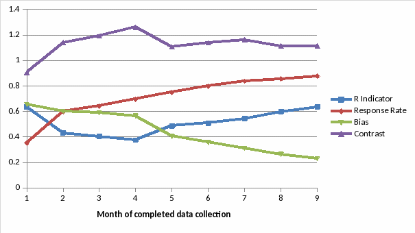
R decreases initially and then increases to end at about the same point as the initial value of R. The bias decreases over time (see table 1 and figure 1).
R and M are not comparable since R is at the group-level and M is at the person-level. We decided not to take the time to simulate M.
We looked at correlations between the model variables and the outcome measures. The bivariate correlations were mostly below .2 and the aggregate correlation was around .4.
We performed two simulations for the computation of R.
Based on partial R’s, targeted base year nonrespondents and hard to locate cases.
First simulation:
Nonrespondents after 3 months of data collection in B&B:09, were classified in the simulation to be final respondents or nonrespondents with their probability of being a respondent or nonrespondent based on their propensity score. This assignment of respondent or nonrespondent was simulated 1,000 times with the results shown below based on the average.
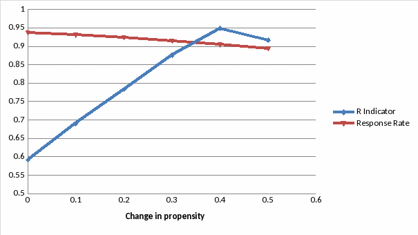
The propensity of the targeted group was increased by 0, 10, 20, 30, 40, and 50 percent. The propensity of the non-targeted groups was decreased by the same percentage (although we do not plan to do this in practice).
R increased as propensity increased up to 40 percent and then decreased (see figure 2).
Second simulation:
Only actual respondents were used, so that outcome measures could be computed.
Nonrespondents in the targeted group after 3 months who became respondents by the end of the 9 month data collection period (n=600), were randomized for this simulation to be classified as final respondents or nonrespondents. This randomization was simulated 500 times with the results shown below based on the average.
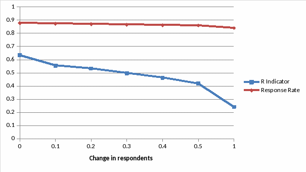
The percentage of the cases that was treated as nonrespondents was varied in the simulations from no cases changing from respondent to nonrespondent up to all targeted cases changing.
R decreased as less cases in the target group were respondents (see figure 3).
3 of 26 outcome measures changed significantly with the target group excluded (see table 2).
B&B:12 full-scale recommendations
We recommend using the R-indicator for B&B:12.
R is good for studies like B&B where there are a lot of data known for respondents and nonrespondents, for which a good model can be developed.
We will monitor R on a regular basis and evaluate R and the partial R’s at three points in data collection to determine how to change the data collection for a targeted group.
We plan to re-visit the model to see what additonal paradata could be added and to explore any additonal variables, including demographics, to add.
The R-indicator cannot be used alone because sample yield targets (based on precision requirements) must also be taken into account during data collection.
We could later explore using an individual-level measure within subgroups to prioritize cases for certain data collection treatments.
Given that we don’t know exactly how well the R-indicator will work to reduce bias and limitations of our simulations, we recommend implementing an experiment.
Experiment plans:
Starting out with a 17,000 sample.
We’re proposing either a 1:3 or 1:1 treatment-to-control ratio (randomly assigned).
Control group will be exposed to the same monetary & non-monetary toolbox as our field-test sample.
Treatment group will be exposed to varied intensity levels of these incentive tools based on their representativeness (partial R-indicator), (e.g. treatment cases in the targeted group will receive the targeted interventions).
Incentive tools include
Date at which outbound calling begins;
Date at which case is sent to intensive tracking and tracing;
Date at which abbreviated interview is offered; and
Monetary incentive increase (base of $20/$35/$50 + added amt of $15).
Table 1. Summary of R-indicator by month – B&B:08/09 data
Month |
R- indicator |
Response rate |
Bias |
Contrast |
Average propensity-overall |
Average propensity - respondents |
Average propensity - nonrespondents |
1 |
0.636 |
0.353 |
0.654 |
0.906 |
0.278 |
0.396 |
0.237 |
2 |
0.432 |
0.599 |
0.602 |
1.140 |
0.472 |
0.643 |
0.329 |
3 |
0.403 |
0.642 |
0.590 |
1.193 |
0.505 |
0.682 |
0.335 |
4 |
0.376 |
0.697 |
0.565 |
1.261 |
0.552 |
0.728 |
0.344 |
5 |
0.486 |
0.750 |
0.406 |
1.105 |
0.633 |
0.731 |
0.467 |
6 |
0.509 |
0.798 |
0.358 |
1.139 |
0.685 |
0.769 |
0.509 |
7 |
0.544 |
0.837 |
0.311 |
1.162 |
0.732 |
0.800 |
0.556 |
8 |
0.597 |
0.855 |
0.264 |
1.114 |
0.763 |
0.815 |
0.606 |
9 |
0.634 |
0.877 |
0.230 |
1.113 |
0.793 |
0.834 |
0.647 |
Figure 1. Summary of R-indicator by month – B&B:08/09 data

Figure 2. Summary of R-indicator by change in propensity - simulation 1

Figure 3. Summary of R-indicator by change in respondents - simulation 2

Table 2. Summary of outcome measures by change in respondents - simulation 2
Outcome measure |
Change in response |
|||
None |
10 percent |
50 percent |
All |
|
Bachelor’s degree major – STEM major |
0.164 (0.158, 0.170) |
0.164 (0.163, 0.165) |
0.164 (0.163, 0.166) |
0.165 (0.164, 0.166) |
Cumulative undergraduate grade point average (multiplied by 100, mean) |
326.252 (325, 327.5) |
326.366 (326.2, 326.5) |
326.843 (326.7, 327) |
327.496 (327.3, 327.7) |
First institution sector – 2-year or less |
0.298 (0.287, 0.31) |
0.299 (0.298, 0.3) |
0.302 (0.301, 0.304) |
0.307 (0.305, 0.308) |
Number of institutions attended before bachelor’s completion |
0.551 (0.538, 0.564) |
0.552 (0.551, 0.554) |
0.558 (0.556, 0.559) |
0.565 (0.563, 0.567) |
Time to 2007-08 bachelor’s degree (mean time in months) |
78.716 (76.8, 80.6) |
78.783 (78.6, 79) |
79.027 (78.8, 79.2) |
79.399 (79.2, 79.6) |
Cumulative total amount borrowed (mean) |
16,299.182 (15,843, 16,755) |
16,390.570 (16,346, 16,435) |
16,770.800 (16,726, 16,815) |
17,302.090 (17,258, 17,346) |
Cumulative amount owed as of 2008-09 (mean) |
15,840.598 (15,365, 16,317) |
15,937.050 (15,890, 15,984) |
16,336.050 (16,289, 16,383) |
16,896.750 (16,850, 16,944) |
Cumulative federal amount borrowed (mean) |
11,304.202 (10,992, 11,616) |
11,355.670 (11,317, 11,394) |
11,569.230 (11,530, 11,608) |
11,867.670 (11,829, 11,906) |
Debt burden in 2008-09 (mean) |
3.408 (3.098, 3.718) |
3.432 (3.393, 3.471) |
3.529 (3.49, 3.567) |
3.668 (3.629, 3.707) |
Ever received Pell grant |
0.372 (0.358, 0.385) |
0.373 (0.371, 0.375) |
0.377 (0.376, 0.379) |
0.383 (0.382, 0.385) |
Loan status in 2008-09 – not repaying |
0.178 (0.168, 0.187) |
0.179 (0.177, 0.18) |
0.182 (0.181, 0.183) |
0.187 (0.186, 0.188) |
Enrollment status in degree program in 2009 – master’s |
0.011 (0.0085, 0.0136) |
0.011 (0.0106, 0.0113) |
0.011 (0.0104, 0.0112) |
0.011 (0.0101, 0.0109) |
Highest degree program enrollment after bachelor’s degree, as of 2009 – master’s |
0.194 (0.184, 0.204) |
0.194 (0.193, 0.195) |
0.194 (0.193, 0.196) |
0.195 (0.194, 0.196) |
Number of jobs held since bachelor’s degree – one |
0.501 (0.489, 0.514) |
0.501 (0.499, 0.503) |
0.500 (0.498, 0.502) |
0.498 (0.496, 0.5) |
Employment status in 2009 – one job |
0.703 (0.692, 0.714) |
0.703 (0.701, 0.704) |
0.703 (0.701, 0.704) |
0.702 (0.701, 0.704) |
Satisfied with employment in 2009 – compensation |
0.558 (0.549, 0.572) |
0.558 (0.556, 0.56) |
0.557 (0.555, 0.559) |
0.556 (0.554, 0.558) |
Employer benefits in 2009 offered medical or health insurance |
0.763 (0.752, 0.774) |
0.762 (0.761, 0.764) |
0.761 (0.76, 0.762) |
0.759 (0.757, 0.76) |
Earned income in 2009 (mean) |
29,139.719 (28,526, 29,753) |
29,099.780 (28,993, 29,206) |
28,949.940 (28,843, 29,057) |
28,731.680 (28,625, 28,838) |
Job not part of career in industry |
0.165 (0.153, 0.177) |
0.165 (0.163, 0.166) |
0.166 (0.164, 0.167) |
0.167 (0.165, 0.168) |
Job unrelated to major |
0.272 (0.259, 0.284) |
0.272 (0.27, 0.273) |
0.273 (0.271, 0.274) |
0.275 (0.273, 0.276) |
Highest education attained by either parent – bachelor’s degree |
0.260 (0.25, 0.271) |
0.260 (0.259, 0.262) |
0.260 (0.259, 0.262) |
0.260 (0.259, 0.262) |
Age at bachelor’s degree receipt (mean) |
25.273 (25.08, 25.46) |
25.278 (25.26, 25.3) |
25.297 (25.28, 25.32) |
25.326 (25.31, 25.35) |
Has disability in 2007-08 |
0.082 (0.075, 0.089) |
0.082 (0.081, 0.083) |
0.082 (0.081, 0.083) |
0.082 (0.081, 0.083) |
Marital status and dependents – unmarried with no dependents |
0.653 (0.64, 0.666) |
0.652 (0.651, 0.654) |
0.650 (0.649, 0.652) |
0.647 (0.646, 0.649) |
Volunteered in last 12 months as of 2009 |
0.409 (0.397, 0.421) |
0.409 (0.407, 0.41) |
0.407 (0.406, 0.409) |
0.406 (0.404, 0.408) |
Ever voted as of 2009 |
0.875 (0.866, 0.883) |
0.875 (0.874, 0.876) |
0.876 (0.875, 0.877) |
0.878 (0.877, 0.879) |
Note: Highlighted variables show a significant difference between the “None” and “All” columns.
1 These findings were originally presented to representatives from NCES and OMB on 2/7/2012. The recommendations in this document have been superseded by those in Part B.
| File Type | application/vnd.openxmlformats-officedocument.wordprocessingml.document |
| Author | Ted Socha |
| File Modified | 0000-00-00 |
| File Created | 2021-01-30 |
© 2026 OMB.report | Privacy Policy