Bobbit - Weighting Scheme
Bobbit - Weighting Scheme.doc
International Price Program U.S. Export and Import Price Indexes
Bobbit - Weighting Scheme
OMB: 1220-0025
K
EY
WORDS: Bootstrap method; Item weights; Secondary classification
system
1. Introduction1
The International Price Program collects data on the United States' trade with foreign nations and publishes monthly indexes on the changes in import and export prices for both merchandise and services. Recently, changes have been recommended in the method of computing item weights for the IPP. These changes are expected to provide a reasonable weight formula, an efficient way to maintain weights, and to improve the weights for the secondary classification systems. The recommended weighting method will be compared to the conventional method according to the magnitude of variance and of the resulting indexes from the two methods. The bootstrap method is the main tool to provide the necessary variance estimates in the study. We will provide the relevant literature review, with special attention to the bootstrap method associated with complex sample designs. We will also present an overview of the IPP sample design and weight structure. Finally, we will describe the comparison study with an emphasis on goodness of fit criteria. The proposed methods are applied to selected subsets of items from the IPP.
2. Background
The International Price Program (IPP) of the Bureau of Labor Statistics (BLS) produces two of the major price statistics for the United States: the Import Price Indexes and the Export Price Indexes. These indexes, in conjunction with the Bureau’s two other monthly price programs -- the Producer Price Indexes (PPI) and Consumer Price Indexes (CPI) -- provide a complete portrait of price trends in the U.S. economy. Import and Export Price Indexes serve a variety of purposes including deflating U.S. trade data, measuring price changes and trends in the foreign sector of the U.S. economy, measuring international competitiveness, and measuring exchange rate effects. The IPP, as the primary source of data on price change in the foreign trade sector of the U.S. economy, publishes monthly indexes on import and export prices of U.S. merchandise and services. IPP currently publishes index estimates of price change for internationally traded goods using three different classification systems - Harmonized System (HS), Bureau of Economic Analysis End Use (BEA), and the Standard International Trade Classification (SITC). IPP also publishes selected transportation indexes and goods indexes based upon the country or region of origin. This paper will only focus on the Import goods indexes that IPP publishes monthly.
The major price programs at the BLS use the following general approach for calculating price indexes. A market basket is sampled to be representative of the universe of prices being measured. Prices for the items in that market basket are then collected from month to month. Using an index methodology that holds quantities fixed, price indexes are derived measuring pure price change as distinct from changes in the product mix.
The target universe of the import and export price indexes consists of all goods and services sold by U.S. residents to foreign buyers (Exports) and purchased from abroad by U.S. residents (Imports). Ideally, the total breadth of U.S. trade in goods and services in the private sector would be represented in the universe. Items for which it is difficult to obtain consistent time span for comparable products, however, such as works of art, are excluded. Products that may be purchased on the open market for military use are included, but goods exclusively for military use are excluded.
3. Sampling in the International Price Program
A sampling frame should mirror the exact universe that the indexes are designed to represent. In the case of the IPP indexes, the Bureau has the luxury of a comparatively good set of sampling frames. The import merchandise sampling frame is obtained from the U.S. Customs Service. The export merchandise sampling frame is a combination of data obtained from the Canadian customs service for exports to Canada and from the Bureau of the Census for exports to the rest of the world. Because shippers are required to document nearly all trade into and out of the U.S., IPP is able to sample from a fairly large and detailed frame; one that, interestingly enough is considerably more detailed and complete than the frames available to either the CPI or the PPI. The frames contain information about all import or export transactions that were filed with the U.S. Customs service during the reference year (or Canadian customs service for exports to Canada). The information available for each transaction includes a company identifier (usually the Employer Identification Number), the detailed product category (Harmonized Tariff number for Imports and the Schedule B number for Exports) of the goods that are being shipped and the corresponding dollar value of the shipped goods.
Starting in 1989, IPP divided the import and export merchandise universes into two halves referred to as panels. Samples for one import half and one export half are selected each year and sent to the field offices for collection, so both universes are fully re-sampled every two years. The sampled products are priced for approximately five years until they are replaced by a fresh sample from the same panel or half-universe. As a result, each published index is based upon the price changes of items from up to three different samples2.
Each panel is sampled every other year using a three stage sample design. The first stage selects establishments independently proportional to size (dollar value) within each broad product category (stratum) identified within the harmonized classification system (HS). An establishment can be selected in more than one stratum.
The second stage selects detailed product categories (classification groups) within each establishment - stratum using a systematic probability proportional to size (PPS) design. The measure of size is the relative dollar value adjusted to ensure adequate coverage for all published strata across all classification systems (HS, BEA, SITC and NAICS3), and known non-response factors (total company burden and frequency of trade within each classification group). Each establishment – classification group (or sampling group) can be sampled multiple times and the number of times each sampling group is selected is then referred to as the number of quotes requested.
In the third and final stage, the BLS Field Economist, with the cooperation of the company respondent, performs the selection of the actual item for use in the IPP indexes. Although the data available from the IPP sampling frame(s) does not provide information about specific items, a detailed product category or classification group description is available to the Field Economist and the respondent, which facilitates the list of items eligible for selection. Beginning with these entry level classification groups and the list of items provided by the respondent to the field economist, further stages of sampling are completed until one item for each quote sampled in the classification group is selected. This process is called disaggregation. This process is done with replacement, so the same item can be selected more than once and the number of instances an item is selected within a sample is referred to as the number of quotes an item represents.
4. Index Estimation
IPP uses the items that are initiated and re-priced every month to compute its indexes of price change. These indexes are calculated using a modified Laspeyres index formula. The modification differs from the conventional Laspeyres in that the IPP uses a chained index instead of a fixed-base index. Chaining involves multiplying an index (or long term relative) by a short term relative (STR). This is useful since the product mix available for calculating indexes of price change can change over time. These two methods produce identical results as long as the market basket of items does not change over time and each item provides a usable price in every period. In reality, the mix of items available at time t is somewhat different than what was available in the base period. In fact, due to non-response, the mix of items used in the index from one period to the next is often different. The benefits of chaining over a fixed base index include a better reflection of changing economic conditions, technological progress, and spending patterns, and a suitable means for handling items that are not traded every calculation month.
Below is the derivation of the modified fixed quantity Laspeyres formula used in the IPP.
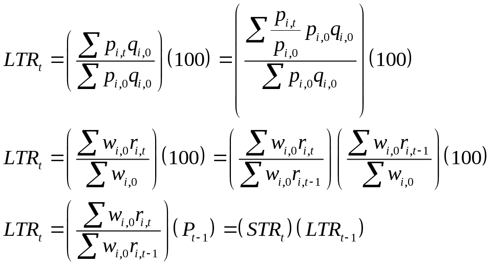
where
LTRt = long term relative of a collection of items at time t
pi,t = price of item i at time t,
qi,0 = quantity of item i in base period 0,
wi,0 = (pi,0)(qi,0) = total revenue of item i, in baseperiod 0,
ri,t = pi,t / pi,0 = long term relative of item i at time t,
![]() = short term relative of a collection of items i, at time t
= short term relative of a collection of items i, at time t
For each classification system, IPP calculates its estimates of price change using an index aggregation structure (i.e. aggregation tree) with the following form:
Upper Level Strata
Lower Level Strata
Classification Groups
Weight Groups (i.e. Company–Index Classification Group)
Items
As mentioned previously, at any given time, the IPP has up to three samples of items being used to calculate each stratum’s index estimate4. Currently the IPP combines the data from these samples by ‘pooling’ the individual estimates. Pooling refers to combining items from multiple samples at the lowest level of the index aggregation tree, in this case, the weight group level. Different sampling groups can be selected for the same weight group across different samples, so it is possible that multiple items from different sampling groups can be used to calculate a single weight group index. An alternative method to pooling is to calculate a ‘composite’ estimate which would calculate a Stratum’s index separately for each sample, and then combine the estimates together across samples at the Stratum level. While this is the more common method, pooling is used by IPP for various practical reasons including the need by Industry Analysts within IPP to see index information across samples at the lowest levels possible for analysis purposes.
5. Aggregation Weights
Up until January of 2004 the weights used to aggregate the item, weight group and classification group indexes to the next level were based upon the sampling weights which reflect the importance that each establishment–classification group was sampled to represent within a particular stratum. The weights used to aggregate the stratum level indexes to the next higher level corresponded to the total dollar value of import or export trade within each stratum as reported by the U.S. Department of Commerce. These weights were based upon a reference year that is 2 years prior to the index calculation year. For example, the indexes that are now calculated for 2005 use weights based upon the trade dollar values from 2003.
Starting in January 2004, IPP changed the aggregation weights used at the classification group level to match what was being used at the stratum levels, which is the total trade dollar value within each classification group. Like the Stratum weights, they are based upon the published dollar values provided by the Department of Commerce and use a reference period that is 2 years old. Prior to making this change, a research group was chartered to explore the impact of this change on IPP’s published indexes as well as to re-evaluate the then current method of calculating item and weight group weights. This paper focuses on the analysis of the item and weight group weights, proposes an alternative approach to calculating the weights and compares test indexes calculated using the new and old weight formulas.
5.1 Item and Weight Group Weight Formulas
Prior to January 2005, the item and weight group weights were defined using the following methodology:
![]()
Where:
Vkh = Quote allocation for sample stratum h from sample k
Qik = Number of quotes represented by selected item i in sample k
Rk = Total number of quotes requested across all sampling groups with that item in sample k
γkjh = Weight of sampling group j from sample k, normalized to sampling stratum h 5
![]()
Where:
Vkh = Quote allocation for sample stratum h from sample k
ωkjh,t= Weight of sampling group j within weight group m at time t, from sample k, normalized to sampling stratum h
The term Vkh was chosen to serve as an inverse proxy of the sampling stratum’s variance. In other words, we assume that strata with higher quote allocations will have lower variances. This term is used to simulate weighted indexes from different samples by the inverse of each indexes variance.
For the adjusted sampling group weight (γkjh), IPP has used a normalized weight to facilitate the combination of sampling weights across samples. Sampling group weights based solely on dollar values would have otherwise introduced an inflation bias into the weight, since items from different samples are based on different reference periods. Normalization within the sampling stratum was originally chosen as a way of avoiding the need to create a complex rebasing system for sampling group Weights.
ωkjh,t differs slightly from the item weight’s γkjh in that it refers to sampling group received, rather than simply the sampling group that was sampled.6 The sampling group received is defined as the establishment – index classification group within a given sample. In some cases, the classification group used for sampling purposes may be different than the classification group used for index estimation. An example of this is computers where the sampling classification group was defined at a more aggregate level than the detailed index classification groups that the computer items are assigned to for estimation purposes. This is done in part to address the highly volatile nature of the computer industry. As a result of this situation, the weight associated with the sampling group is split among the more detailed establishment – index classification groups based upon the make-up of the computer items that were selected during disaggregation. Unlike γkjh, which is static, ωkjh,t can change over time as items are reclassified to different index classification groups. IPP evaluates the index classification groups each year and redefines them to account for changes to the more detailed Harmonized Tariff or Schedule B numbers. This is one example of the why maintaining a separate set of weight group weights can be somewhat complex. During the term of a single sample’s repricing as items are reclassified to the appropriate index classification group, or as new sampling groups are initiated, or as companies are redefined due to splits and mergers, weight group weights change accordingly.
After examining the current methodology, the group identified the following issues that needed to be addressed:
The normalization of the sampling weights to strata within the Harmonized System can result in inappropriate weights in the secondary classification systems. (i.e. BEA, SITC, NAICS)
There had been an operational concern within the program for some time about the various systems that were needed to maintain weight group weights and it was thought that redefining the item weights so that they would sum to the weight group weight would eliminate the complex system that exists for maintaining weight group level weights. Weight group weights can change any time there is a change in the sampling group mix within the weight group. They can also change whenever there is a change in the index classification group or the company identifier for an item, which can cause the item to switch weight groups.
5.2 Recommended Changes
The group proposed addressing these concerns by 1) Rebasing the adjusted sampling group weights to the same reference period, instead of normalizing. This would allow the weights to be combined in a meaningful way across all classification systems. 2) Re-define the formula for the item weights so that they will sum to the weight group weights. Item weights will need to be recalculated each month to account items that have been discontinued. The specific recommended changes are as follows:
Abandon the practice of normalizing the sampling group weights, in favor of rebasing adjusted sampling group weights to the same reference period (index base year). γkj is redefined to be:
![]()
where:
wkj = Adjusted (but not normalized) weight for sampling group j from sample k
![]() kj-base
year = The average of all LTRs in the 12 months of index base
year
kj-base
year = The average of all LTRs in the 12 months of index base
year
![]() kj-sample
ref. period = The average of LTRs during the 12 months of the
sample reference period
kj-sample
ref. period = The average of LTRs during the 12 months of the
sample reference period
Use the following item weight formula, which will need to be recalculated monthly to adjust for discontinued items within a sampling group (non-response).
![]()
where:
Qik = Number of quotes represented by item i in sample k
Ak,t = # non-discontinued (active) items at time t, across all sampling groups with that item in sample k.
γkj = Weight of sampling group j from sample k rebased to the index base year.
The weight group weight will be the sum of these item weights for the set of non-discontinued items within the weight group (Company–index classification group) for the given month. We no longer have to worry about calculating a separate sampling group received weight since the items are summed up to calculate a weight for the weight group that each item is associated with in the current period.
Drop the Vkh term in the current item weight formula. This is not needed since the sampling group weights are no longer normalized.
A study was conducted to evaluate the results of the proposed changes. Test indexes were calculated using the old item and weight group weight formulas, as well as the revised formulas which incorporated the proposed changes. Comparisons were based upon bootstrap estimates of the bias and variance of the index estimates.
6. Comparison study
The two weighting schemes outlined in sections 5.1 and 5.2 above were
applied to 150 bootstrap samples. These bootstrap samples were drawn
with replacement from a comprehensive list of all items belonging to
a full sample for each of the months from February 2003 to January
2005. Bootstrap weights were then computed at the item level, for
both weighting methods. The short term index values (STR) (define
![]() to be the STR values calculated using the old weighting method;
to be the STR values calculated using the old weighting method;
![]() the STR values calculated using the new weighting method) were then
computed for each bootstrap sample using both the new and old
weighting methods. We computed these repeated estimates of
the STR values calculated using the new weighting method) were then
computed for each bootstrap sample using both the new and old
weighting methods. We computed these repeated estimates of
![]() and
and
![]() for the following strata:
for the following strata:
HS
All imports
P8473 (Computer parts) – This strata is also very volatile with some seasonality.
BEA
All imports
R21320 (Semiconductors)—This strata is volatile, and contains items from two different Harmonized 4-digit strata
6.1 Literature Review
We used a bootstrap method to compute estimates for variance and bias in our weight comparison study. We compared different weighting schemes according to the magnitude of these estimates.
Other well-known resampling methods are the jackknife and balanced repeated replication (BRR). However the bootstrap is considered the most flexible method among them. One of the reasons for this is that the jackknife and the BRR methods are applicable only to those stratified multistage designs in which clusters within strata are sampled with replacement or the first-stage sampling fraction is negligible (Rao et al., 1992).
Since Efron (1979) proposed his bootstrap method, the bootstrap method for the iid case has been extensively studied. The original bootstrap method was then modified to handle complex issues in survey sampling, and results were extended to cases such as stratified multistage designs. Rao and Wu (1987) provided an extension to stratified multistage designs but covering only smooth statistics. Later, Rao et al (1992) extended the result to non-smooth statistics such as the median by making the scale adjustment on the survey weights rather than on the sampled values directly. The main technique which was used to apply the bootstrap method to complex survey data is scaling. The estimate of each resampled cluster is properly scaled so that the resulting variance estimator reduces to the standard unbiased variance estimator in the linear case (Rao and Wu, 1987). Sitter (1992) explored the extensions of the bootstrap to complex survey data and proposed a mirror-matched bootrap method for a variety of complex survey designs. Sitter mentioned in his study that it was difficult to compare the performances of his proposed method with those in Rao and Wu (1988)'s rescaling method either theoretically or via simulation.
6.2 Implementation issues
The following is a list of differences between the test indexes that were calculated as part of this study and IPP’s published indexes produced in the current production environment.
Prices for a small percentage of the published strata are collected using secondary sources and are not sampled (e.g. Petroleum). We chose to ignore these prices for the purpose of this study.
IPP recently instituted an imputation method referred to as linear interpolation which fills in missing prices using the linear difference between two real prices on either side of the missing price(s). IPP recalculates and revises its published indexes for three consecutive months after the initial published index, which makes this method of imputation useful. For situations that don’t meet the above criteria, missing prices are imputed using the average change of the parent index (cell mean). This study only produced test indexes using the cell mean method of imputation.
Finally, there are a number of relationships in the IPP data that are only stored as static values (e.g. Company identifier, index usable flag). These can change over time. For the purpose of this study, we only used the current values of the data elements so past changes to these values were not accurately reproduced in the data.
6.3 Sample Design Approximations
Section 3 summarized the stratified multistage design used to select
individual items for price quotes that are subsequently incorporated
in the estimator
![]() .
However, we will base our bootstrap resampling procedure on an
approximation to the original complex design. Specifically, we will
approximate the true design with a simplified design that uses the
same strata as in the original design; that treats the individual
items as the PSU selected with replacement and with selection
probabilities proportional to the inverse of their sample weights.
Thus, this "variance approximation design" does not account
directly for the multistage structure in the original design. For
literature on other variance approximation designs that do not
account for the original PSU structure, see, e.g., Korn and Graubard
(1995) and references cited therein.
.
However, we will base our bootstrap resampling procedure on an
approximation to the original complex design. Specifically, we will
approximate the true design with a simplified design that uses the
same strata as in the original design; that treats the individual
items as the PSU selected with replacement and with selection
probabilities proportional to the inverse of their sample weights.
Thus, this "variance approximation design" does not account
directly for the multistage structure in the original design. For
literature on other variance approximation designs that do not
account for the original PSU structure, see, e.g., Korn and Graubard
(1995) and references cited therein.
Due
to the simplified design approximation described above, we will
simplify our notation through omission of the original PSU label c.
Thus, for this section, define
![]() as a sample item i in the stratum h,
as a sample item i in the stratum h,
![]() as the total number of sampled items i in the stratum h,
and
as the total number of sampled items i in the stratum h,
and
![]() as the weight of a sample item i in the stratum h.
as the weight of a sample item i in the stratum h.
Section
5 described a complex procedure for calculation of the weights symbol
used in computation of the original full-sample STR index estimator
![]() .
This weighting procedure incorporated selection probabilities, as
well as other adjustments. For the purposes of the current bootstrap
procedure, we treated the weights as fixed. Consequently, this
bootstrap method will not account explicitly for the additional
components of variability associated with the steps, and the
dependence of these additional steps on the other units included in
the sample.
.
This weighting procedure incorporated selection probabilities, as
well as other adjustments. For the purposes of the current bootstrap
procedure, we treated the weights as fixed. Consequently, this
bootstrap method will not account explicitly for the additional
components of variability associated with the steps, and the
dependence of these additional steps on the other units included in
the sample.
6.4 Bootstrap variance estimator
The following is a detailed description on how we implemented bootstrap sampling for this study.
Draw
 items with replacement from the
 sample
items in each stratum. Let
 be
the number of times that the item i in stratum h is
selected in the bootstrap procedure so that
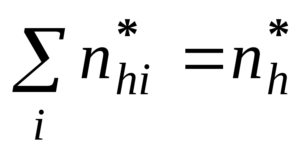 .
In addition we required that
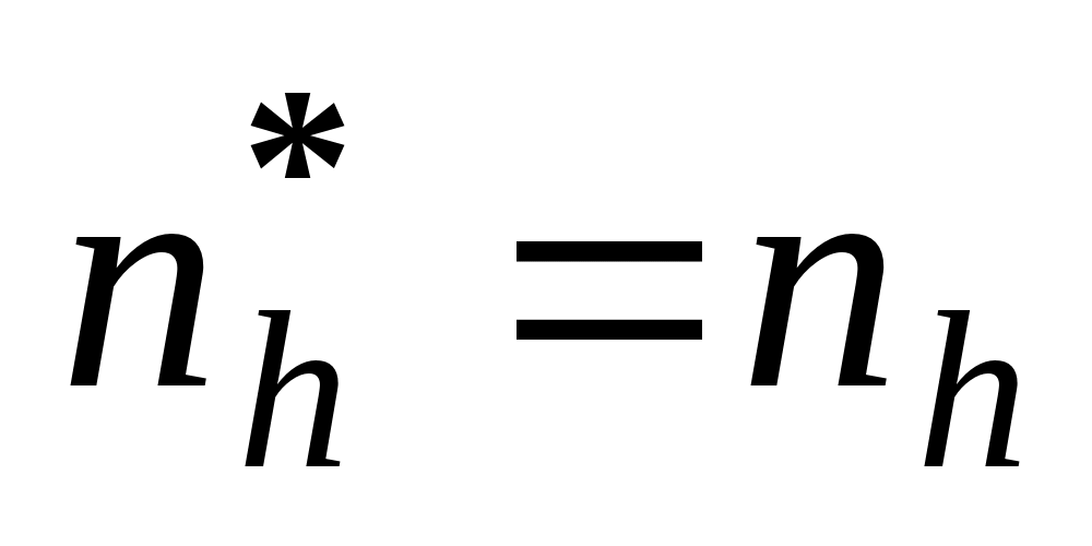 .
.
Define bootstrap weights
 7.
7.Calculate the price STR index using bootstrap weights.
Repeat this process 150 times.
Compute the bootstrap variance estimator,
 ,
using
 where
where
 ,
,
 is a bootstrap STR estimator and
 is the STR estimator from the original sample.
6.5 Goodness of fit criteria
We considered the following test statistics from the different weighting schemes.
For
each month t, let
![]() be a bootstrap variance estimator from a new weighting scheme.
Where
be a bootstrap variance estimator from a new weighting scheme.
Where![]() is the STR index estimator from the original sample computed using
the new weighting method. Similarly, let
is the STR index estimator from the original sample computed using
the new weighting method. Similarly, let
![]() be a bootstrap variance estimator from an old weighting scheme. Where
be a bootstrap variance estimator from an old weighting scheme. Where
![]() is the STR index estimator from the original sample computed using
the new weighting method. For each month t, we compared STR
estimators from the old and new methods relative to old STR
estimator:
is the STR index estimator from the original sample computed using
the new weighting method. For each month t, we compared STR
estimators from the old and new methods relative to old STR
estimator:
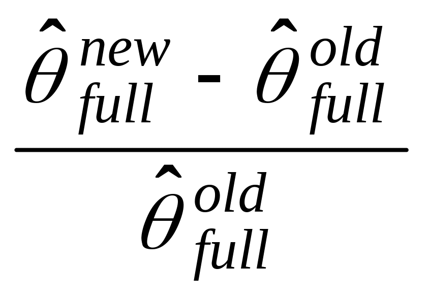 (1)
(1)
then we checked whether the change was large relative to old standard error:
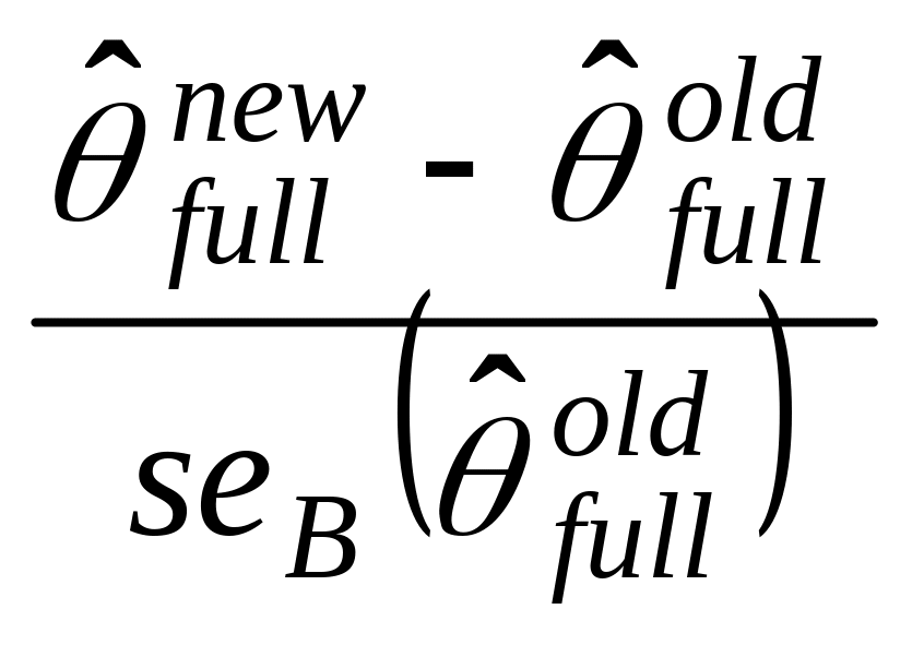 (2)
(2)
where
![]() ,
,
we then examined the statistical significance of the following test statistic:
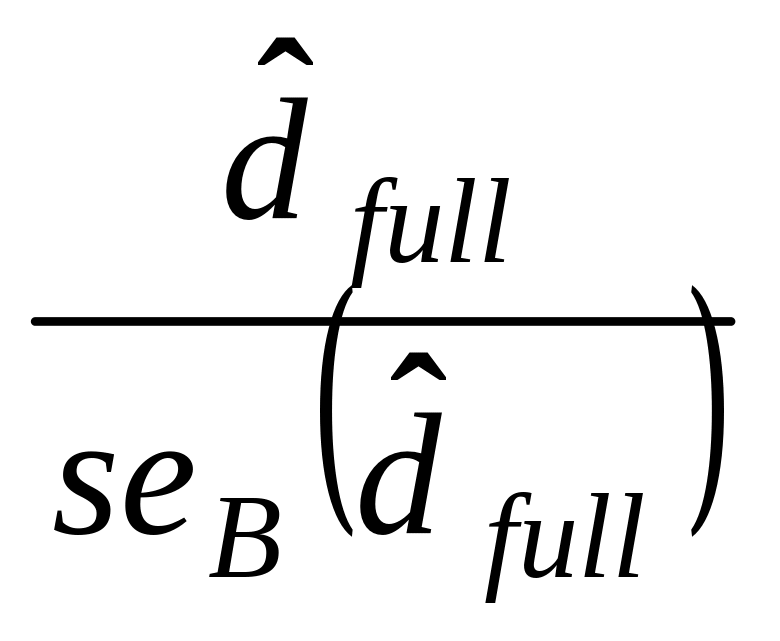 (3)
(3)
where
![]() ,
,
![]() ,
,
![]() ,
,
![]() .
.
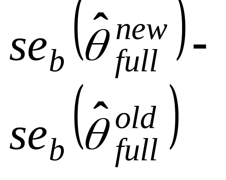
finally, we compared the estimated precision by comparing
![]() with
with
![]() (4).
(4).
6.6 Results
Figure
1 gives an overview of the bootstrap data. In the figure, the blue
crosses represent the individual bootstrap replicate STR indexes![]() .
The red triangle is the mean of the replicate STR indexes
.
The red triangle is the mean of the replicate STR indexes ,
the green dots are the values actually published at the time, and the
yellow dots are the estimates obtained from the full sample data
![]() .
The data is repeated new/old for each period allowing for a direct
comparison. Similar plots for other more specific strata are included
in the appendix.
.
The data is repeated new/old for each period allowing for a direct
comparison. Similar plots for other more specific strata are included
in the appendix.
Points of interest in this plot
There appears to be little difference between the two weighting schemes in the ‘spread’ of the bootstrap replications, and their mean estimates.
While there seem to be noticeable differences between the yellow (index estimate using the full sample) and green (published index) these are explained by variations in the implementation of the estimation programs outlined in the discussion section below.
Since our chain started in Febuary 2003, we fixed our estimate (yellow dot, red triangle) to be 1 to avoid scaling issues.
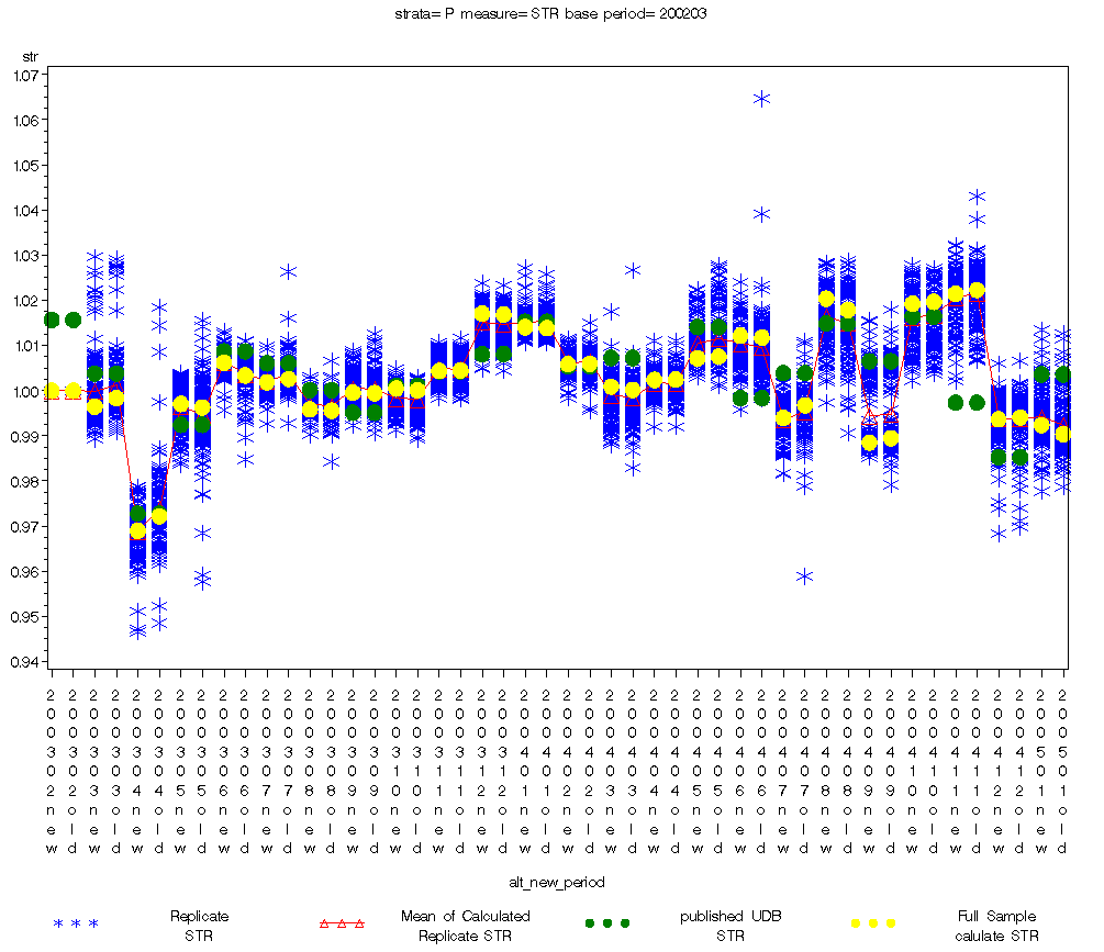
Figure 1: Bootstrap Data for All Imports
6.6.1 All Imports (HS)
When we compared STR differences between the old and new methods with respect to Old-STR, there were no STR differences that exceeded 0.5% of Old-STR for all 23 months (see Table 1). Similarly, for all 23 months, the mean of the STR didn’t exceed one standard error (SE) of the mean, nor were any of the test statistics significant.
Table 1: Goodness of fit statistics, All imports |
||||
Period |
Relative Diff.
(1) |
Mean as % of SE
(2) |
Test Statistic For Diff of Means (3) |
(4) |
Mar-03 |
-0.0019 |
-0.2231 |
-1.1534 |
-0.0002 |
Apr-03 |
-0.0033 |
-0.3685 |
-0.3978 |
-0.0035 |
May-03 |
0.0008 |
0.0990 |
0.1258 |
-0.0035 |
Jun-03 |
0.0028 |
0.7227 |
0.8199 |
-0.0015 |
Jul-03 |
-0.0007 |
-0.1974 |
-0.1903 |
-0.0014 |
Aug-03 |
0.0003 |
0.1051 |
0.1433 |
-0.0008 |
Sep-03 |
0.0001 |
0.0238 |
0.0453 |
-0.0008 |
Oct-03 |
0.0004 |
0.1142 |
0.2914 |
0.0000 |
Nov-03 |
-0.0001 |
-0.0334 |
-0.1081 |
-0.0001 |
Dec-03 |
0.0002 |
0.0479 |
0.1759 |
-0.0003 |
Jan-04 |
0.0002 |
0.0689 |
0.1774 |
-0.0002 |
Feb-04 |
-0.0001 |
-0.0365 |
-0.0747 |
-0.0005 |
Mar-04 |
0.0007 |
0.1288 |
0.2661 |
-0.0005 |
Apr-04 |
-0.0001 |
-0.0338 |
-0.0762 |
-0.0002 |
May-04 |
-0.0004 |
-0.0584 |
-0.1859 |
-0.0014 |
Jun-04 |
0.0004 |
0.0535 |
0.0676 |
-0.0025 |
Jul-04 |
-0.0028 |
-0.4828 |
-0.6121 |
-0.0021 |
Aug-04 |
0.0025 |
0.3230 |
0.6539 |
-0.0003 |
Sep-04 |
-0.0010 |
-0.1013 |
-0.3188 |
0.0001 |
Oct-04 |
-0.0004 |
-0.0643 |
-0.3009 |
0.0003 |
Nov-04 |
-0.0008 |
-0.1374 |
-0.1759 |
-0.0002 |
Dec-04 |
-0.0004 |
-0.0751 |
-0.2038 |
-0.0003 |
Jan-05 |
0.0020 |
0.3182 |
0.7358 |
-0.0001 |
6.6.2 Computer Parts (HS)
When we compared STR differences between the old and new methods with respect to Old-STR, between the two methods, none exceeded 1% of the Old-STR across all 23 months. All STR differences were less than 0.5% of Old-STR except for 3 months, April and July 2003 and April 2004 (see Table 2). None of the bootstrap means exceeded the SE of the mean, similarly, none of the test statistics were significant. When we compared the estimated precision between two methods, SEs of the New-STR were smaller than the Old-STR in 14 out of 23 months
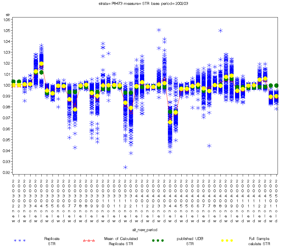
Figure 2: Bootstrap Data for Computer Parts
Table 2: Goodness of fit statistics, Computer Parts |
||||
Period |
Relative Diff.
(1) |
Mean as % of SE
(2) |
Test Statistic For Diff of Means (3) |
(4) |
Mar-03 |
-0.0002 |
-0.1130 |
-0.0929 |
0.0005 |
Apr-03 |
-0.0070 |
-0.8459 |
-1.1721 |
-0.0014 |
May-03 |
0.0026 |
0.8406 |
1.1691 |
-0.0004 |
Jun-03 |
0.0004 |
0.2999 |
0.1969 |
0.0012 |
Jul-03 |
0.0096 |
0.9211 |
1.3350 |
-0.0017 |
Aug-03 |
-0.0008 |
-0.5841 |
-0.7546 |
-0.0006 |
Sep-03 |
0.0025 |
0.2333 |
0.3798 |
-0.0012 |
Oct-03 |
-0.0002 |
-0.0474 |
-0.0373 |
0.0022 |
Nov-03 |
0.0004 |
0.4582 |
0.2681 |
0.0006 |
Dec-03 |
0.0048 |
0.3681 |
0.4903 |
-0.0004 |
Jan-04 |
-0.0035 |
-0.3789 |
-0.6254 |
-0.0022 |
Feb-04 |
0.0003 |
0.3637 |
0.3255 |
0.0003 |
Mar-04 |
-0.0012 |
-0.1220 |
-0.2243 |
-0.0031 |
Apr-04 |
-0.0091 |
-0.8093 |
-0.8363 |
0.0053 |
May-04 |
0.0000 |
0.0000 |
0.0000 |
0.0004 |
Jun-04 |
-0.0012 |
-0.2866 |
-0.4346 |
-0.0014 |
Jul-04 |
0.0023 |
0.2413 |
0.2912 |
-0.0012 |
Aug-04 |
0.0007 |
0.0987 |
0.1206 |
-0.0037 |
Sep-04 |
-0.0011 |
-0.1075 |
-0.1828 |
-0.0006 |
Oct-04 |
-0.0015 |
-0.3436 |
-0.3864 |
-0.0002 |
Nov-04 |
-0.0003 |
-0.2741 |
-0.2705 |
0.0000 |
Dec-04 |
-0.0010 |
-0.1992 |
-0.2898 |
-0.0001 |
Jan-05 |
-0.0005 |
-0.1870 |
-0.1829 |
0.0005 |
6.6.4 All Imports (BEA)
When we compared STR differences between the old and new methods with respect to Old-STR, there were no STR differences that exceeded 1.5% of Old-STR for all 23 months (see Table 3). Similarly, for all 23 months, the mean of the STR didn’t exceed one SE of the mean, nor were any of the test statistics significant. When we compared the estimated precision between two methods, SEs of the New-STR were smaller than the Old-STR in 17 out of 23 months
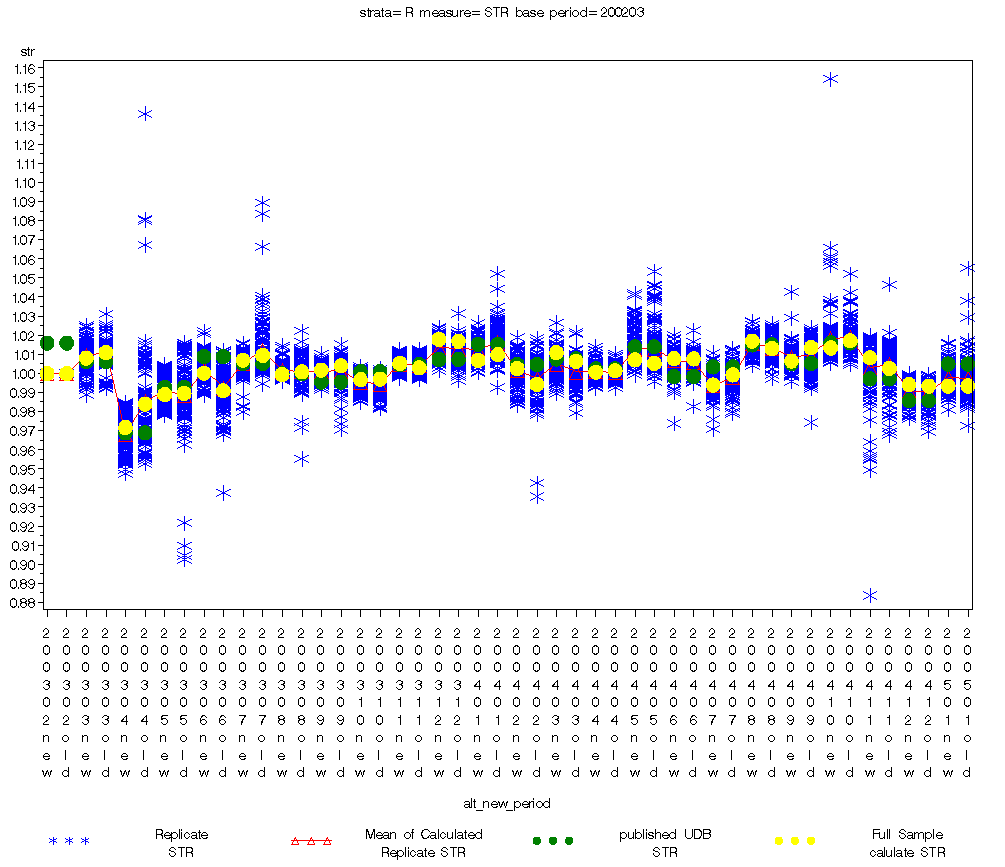
Figure 3: Bootstrap Data for All Imports (BEA)
Table 3: Goodness of fit statistics, All imports |
||||
Period |
Relative Diff.
(1) |
Mean as % of SE
(2) |
Test Statistic For Diff of Means (3) |
(4) |
Mar-03 |
-0.0029 |
-0.4559 |
-0.3019 |
0.0006 |
Apr-03 |
-0.0125 |
-0.5032 |
-0.4556 |
-0.0142 |
May-03 |
-0.0006 |
-0.0330 |
-0.0296 |
-0.0101 |
Jun-03 |
0.0093 |
0.8478 |
0.7296 |
-0.0042 |
Jul-03 |
-0.0025 |
-0.1862 |
-0.1646 |
-0.0075 |
Aug-03 |
-0.0014 |
-0.1933 |
-0.1749 |
-0.0034 |
Sep-03 |
-0.0023 |
-0.3285 |
-0.2986 |
-0.0033 |
Oct-03 |
-0.0003 |
-0.0561 |
-0.0477 |
-0.0008 |
Nov-03 |
0.0023 |
0.5452 |
0.3884 |
-0.0003 |
Dec-03 |
0.0010 |
0.1423 |
0.1250 |
-0.0006 |
Jan-04 |
-0.0030 |
-0.3011 |
-0.3180 |
-0.0022 |
Feb-04 |
0.0084 |
0.7729 |
0.6175 |
-0.0036 |
Mar-04 |
0.0046 |
0.5316 |
0.5136 |
0.0001 |
Apr-04 |
-0.0008 |
-0.2565 |
-0.1537 |
0.0008 |
May-04 |
0.0019 |
0.1405 |
0.1295 |
-0.0034 |
Jun-04 |
0.0001 |
0.0202 |
0.0158 |
0.0008 |
Jul-04 |
-0.0053 |
-0.8937 |
-0.6789 |
-0.0005 |
Aug-04 |
0.0039 |
0.7006 |
0.5261 |
-0.0009 |
Sep-04 |
-0.0070 |
-0.8341 |
-0.6453 |
-0.0028 |
Oct-04 |
-0.0037 |
-0.5570 |
-0.2280 |
0.0090 |
Nov-04 |
0.0056 |
0.5131 |
0.2780 |
0.0059 |
Dec-04 |
0.0008 |
0.1224 |
0.1022 |
-0.0003 |
Jan-05 |
-0.0001 |
-0.0094 |
-0.0084 |
-0.0027 |
6.6.5 Semiconductors (BEA)
When we compared the STR differences between the old and new methods with respect to Old-STR, between the two methods, none exceeded 2% of Old-STR across 23 months. All STR differences were less than 1% of the Old-STR except for three months, July, September and December 2003 (see table 4). When we checked whether the STR differences were large with respect to the SE of Old-STR, the STR differences were less than the SE of Old-STR for 18 out of 23 months. None of the test statistics were significant. When we compared the estimated precision between two methods, SEs of the New-STR were smaller than the Old-STR in 9 out of 23 months
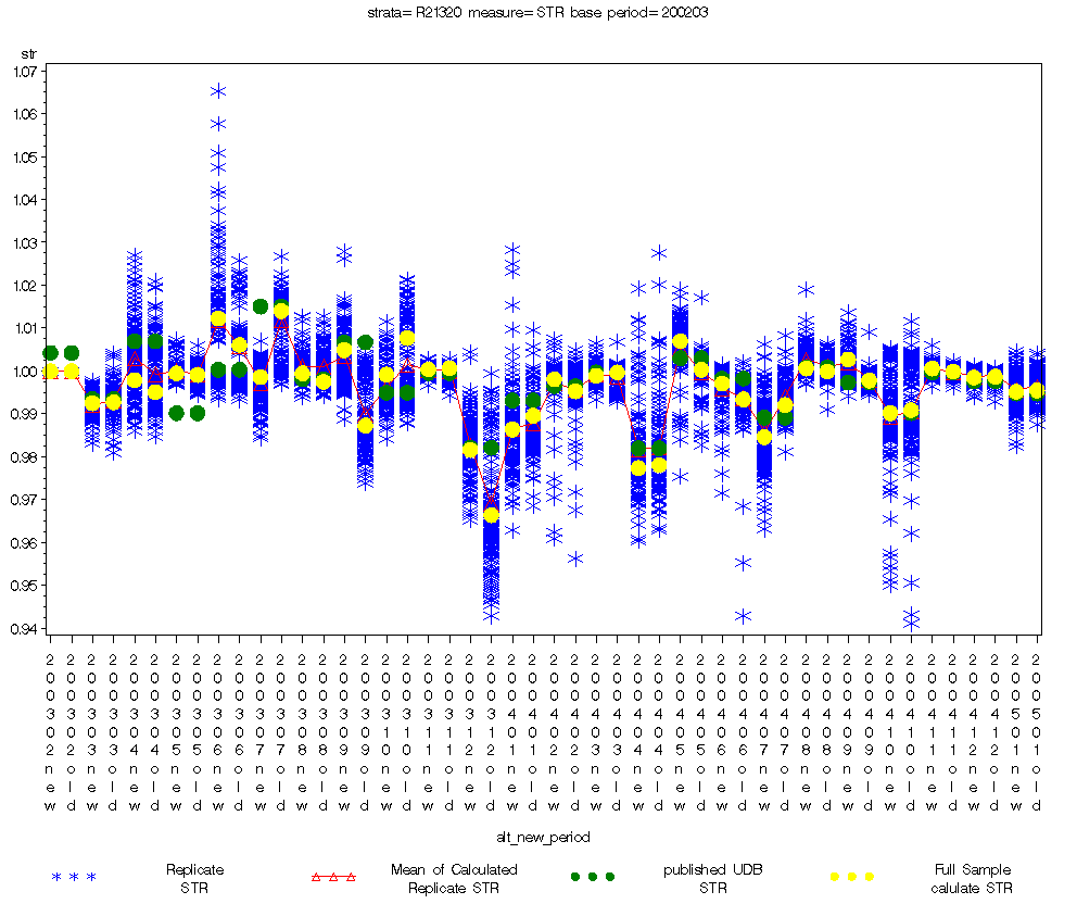
Figure 2: Bootstrap Data for Semiconductors (BEA)
Table 4: Goodness of fit statistics, Semiconductors |
||||
Period |
Relative Diff.
(1) |
Mean as % of SE
(2) |
Test Statistic For Diff of Means (3) |
(4) |
Mar-03 |
-0.0002 |
-0.0574 |
-0.0428 |
-0.0007 |
Apr-03 |
0.0028 |
0.3231 |
0.2479 |
0.0014 |
May-03 |
0.0004 |
0.1927 |
0.1317 |
0.0000 |
Jun-03 |
0.0062 |
0.7305 |
0.3832 |
0.0055 |
Jul-03 |
-0.0152 |
-2.3225 |
-1.8722 |
-0.0019 |
Aug-03 |
0.0020 |
0.3797 |
0.3735 |
-0.0019 |
Sep-03 |
0.0178 |
2.0200 |
1.5267 |
-0.0021 |
Oct-03 |
-0.0084 |
-0.7710 |
-0.7928 |
-0.0053 |
Nov-03 |
-0.0003 |
-0.2125 |
-0.1967 |
-0.0005 |
Dec-03 |
0.0157 |
1.0529 |
0.9921 |
-0.0074 |
Jan-04 |
-0.0032 |
-0.4917 |
-0.2744 |
0.0029 |
Feb-04 |
0.0028 |
0.4620 |
0.3245 |
0.0002 |
Mar-04 |
-0.0008 |
-0.3003 |
-0.2593 |
-0.0008 |
Apr-04 |
-0.0007 |
-0.0645 |
-0.0490 |
0.0005 |
May-04 |
0.0067 |
1.5997 |
0.9063 |
0.0024 |
Jun-04 |
0.0037 |
0.5643 |
0.4746 |
-0.0019 |
Jul-04 |
-0.0076 |
-1.6931 |
-0.8680 |
0.0033 |
Aug-04 |
0.0007 |
0.2633 |
0.1704 |
0.0010 |
Sep-04 |
0.0049 |
3.2084 |
1.2402 |
0.0020 |
Oct-04 |
-0.0007 |
-0.0669 |
-0.0455 |
0.0004 |
Nov-04 |
0.0007 |
0.6497 |
0.3864 |
0.0003 |
Dec-04 |
-0.0002 |
-0.1613 |
-0.1119 |
0.0001 |
Jan-05 |
-0.0003 |
-0.0902 |
-0.0595 |
0.0009 |
6.7 Discussion
That the change in weight did very little to affect the indexes was to be expected. This is because the change from normalization to rebasing was for all intents and purposes a scaling change. That is, in the normalization method, we were forcing the sum of all the weights within a sample stratum to sum to one (by dividing each sample group weight by the total of the weight of all sampling groups within the sampling stratum). Comparing this to the new ‘rebasing’ method, we were simply allowing the dollar values to be added without the effects of time. The difference between the two sums would be very nearly a factor that is equal to the weight-group weight sum.
The change in using only the non-discontinued items would give us very nearly the same total weight (at the weigh-group level) as we would have gotten before.
References
Bureau of Labor Statistics (1997). BLS Handbook of Methods. Washington, DC: U.S. Department of Labor.
The IPP Lower Level Weights Team (2004), Lower Level Weights Proposal.
Efron, B., and Tibshirani, R.J. (1993). An Introduction to the Bootstrap. Chapman & Hall.
Korn, E. and Graubard, B (1995). “Analysis of Large Health Surveys: Accounting for the Sampling Design,” Journal of the Royal Statistical Society, Series A, vol. 158, No. 2, pp. 263-295.
Lahiri, P. (2003). On the impact of bootstrap in survey sampling and small-area estimation. Statistical Science, vol.18, No. 2, pp. 199-210.
Rao, J. and Wu, C. (1988). “Resampling Inference with Complex Survey Data,” Survey Methodology, vol. 83, pp. 231-241.
Rao, J., Wu, C. and Yue, K. (1992). “Some Recent Work on Resampling Methods for Complex Surveys,” Survey Methodology, vol. 18, pp. 209-217.
Rizzo, L. (1986). “Composite Estimation in the International Price Program. Proceedings of the Section on Survey Research Methods,” American Statistical Association, pp. 448-453.
Sitter, R. (1992). “A Resampling Procedure for Complex Survey Data,” Journal of the American Statistical Association, vol. 87, pp. 755-765.
Wolter, K. (1979), “Composite Estimation in Finite Populations,” Journal of the American Statistical Association, vol. 74, num 367, pp. 604-613.
1 Opinions expressed in this paper are those of the authors and do not constitute policy of the Bureau of Labor Statistics. The authors thank Andrew Cohen, John Eltinge, Helen McCulley, Steve Paben and Daryl Slusher at BLS for helpful comments on the International Price Program. The views expressed in this paper are those of the authors and do not necessarily reflect the policies of the U.S. Bureau of Labor Statistics.
2 Indexes for published strata that cross panels, may be based upon items from up to six samples at any one time
3 While IPP does not currently publish indexes by the NAICS classification system, the sampling methodology is designed to ensure enough quotes are available for IPP to begin publishing indexes at some future date in this classification system.
4 Indexes for published strata that cross panels, may be based upon items from up to six samples at any one time.
5
![]() is the normalized value of
is the normalized value of
![]() ,
where Πkj is the probability of selecting
sampling group j from sampling stratum h in sample k.
,
where Πkj is the probability of selecting
sampling group j from sampling stratum h in sample k.
6 Sampling Group Received corresponds to the sample - establishment - index classif group.
7
Rao et al. originally defined bootstrap weights
 where
where
![]() equals
the number of times that the hc-th sample cluster is selected
in the bootstrap re-sampling procedure, and
equals
the number of times that the hc-th sample cluster is selected
in the bootstrap re-sampling procedure, and
![]() if hc-th sample cluster is not selected in the bootstrap
procedure. We chose to define them as
if hc-th sample cluster is not selected in the bootstrap
procedure. We chose to define them as
![]() for computational simplicity.
for computational simplicity.
| File Type | application/msword |
| File Title | The sample design used for this variance research matches the IPP products sample design at the first stage, but simplifies th |
| Author | Gegner_S |
| Last Modified By | Nora Kincaid |
| File Modified | 2009-08-19 |
| File Created | 2009-08-19 |
© 2026 OMB.report | Privacy Policy

