0990-Menu Labeling OMB Supporting Statement Part B_OMB Comment April 13 2016 clean
0990-Menu Labeling OMB Supporting Statement Part B_OMB Comment April 13 2016 clean.docx
Examining Consumer and Producer Responses to Restaurant Menu Labeling Requirements
OMB: 0990-0445
Examining Consumer Responses to Restaurant Menu Labeling Requirements
OMB No. OS-0990-XXXX
Supporting Statement – Section B
Submitted: October 13, 2015, revised March 16, 2016, revised April 12, 2016
Program Official/Project Officer
Amber Jessup, Ph.D.
Senior Economist
U.S. Department of Health and Human Services
Office of the Assistant Secretary for Planning and Evaluation
200 Independence Avenue SW, Washington DC 20201
(202) 690-6621
SUPPORTING STATEMENT
Examining Consumer Responses to Restaurant Menu Labeling Requirements
B. Collection of Information Employing Statistical Methods
1. Respondent Universe and Respondent Selection
This project uses the American Life Panel (ALP) for this project. The American Life Panel (ALP) is a high quality sample with national representativeness. While ALP has been used for national estimates, national representativeness is not required in this study, whose primary aims is how people respond to menu labeling in different settings. Nevertheless, external validity is increased by sampling from a nationally representative sample than a convenience sample as for most internet panel
We will use a random sample of ALP participants (see below for exact numbers). There is no oversampling.
ALP recruits participants from several sources, including the University of Michigan Monthly Survey, the National Survey Project cohort, and several targeted recruitment methods to add specific populations (e.g. active recruitment for vulnerable populations). Such recruitment methods include address-based sampling. Computer ownership or Internet access was not a requirement for ALP in order to eliminate the bias found in other Internet survey panels. For individuals without their own internet access, RAND provides panel members with Internet access by providing a WebTV and an Internet subscription.
Power Calculation
The sample size (2000 completed responses) was determined by the budget. Nevertheless, we conducted power calculations to confirm that this would be sufficient to detect meaningful effects of menu labeling, based on a review of sample sizes and variances in prior field and experimental studies. Power calculations are inherently speculative and no previous work can directly inform this experiment. The best source is a review of quasi-experimental and actual experimental studies (Sinclair et al., 2014). Our best guess of a mean population effect of labeling calories with contextual information across a variety of settings is 67.
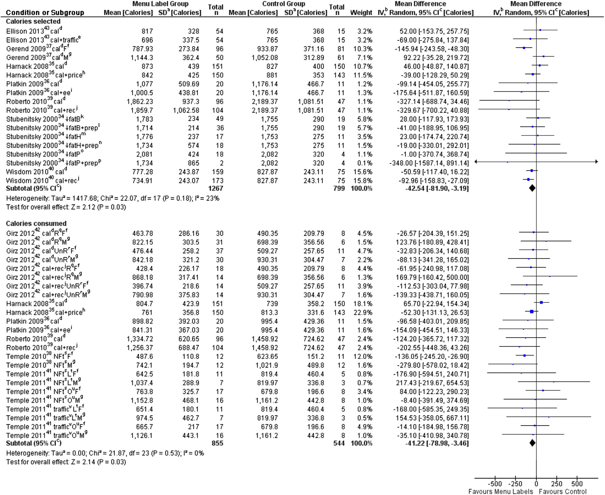
Next, we need to get an estimate about likely variances or standard deviation in responses. The table below summarizes previous experiments. The last column shows the confidence intervals and also indicates the problem with sample sizes in prior studies: Confidence intervals are very wide in studies with 30-300 participants total. Wisdom et al. is an outlier with unusually small confidence intervals despite the small sample.
Table: Summary of Experimental Studies on Menu Labeling
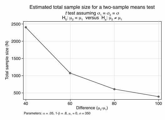
Our first calculation shows what sample sizes are needed for detecting various effects with acceptable power, using a two-sample comparison (Figure 1). We use a standard deviation of 350 calories, about the pooled value in Ellison et al. (2013) or Gerend et al. (2009), which is smaller than the studies by Harnack and Platkin, but larger than Stubenitsky and Wisdom. The calculations are for a two-sided two-sample test with alpha=0.05 and 80% power. N is the combined sample size, so 1000 would be for two groups of 500 each and would have good power to detect the mean effect of 67 kcals. That means we would have good statistical power for comparing 4 subgroups within each setting. Probably we have better power for comparing each of those subgroups across settings, which would be a pairwise comparison as the same individual is considered twice and much of the variation in food choices is between rather than within individuals.
Figure 1: Total sample sizes needed for 80% power as a function of effect size1

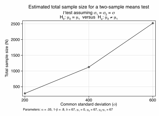
We expect that the standard deviation depends highly on the range of menu options and increases with a broader range of options and decreases with a smaller range. A setting like Starbucks would see smaller variances than Outback Steakhouse. However, we have no data that would allow us to relate the variance in calories in the menu to the variance in calories of choices. So our next calculation is about the influence of variances. We assume the true mean effect is 67 cals and calculate sample sizes when standard deviation across settings range from 200 to 600 kcals. We can see that for settings with very low variation, subsample analysis for small subgroups will be feasible. However, in settings were the standard deviations in individual choices reaches 600, even our full data set will be insufficient to detect the mean effect of 67 (with acceptable power).
Those calculations are only illustrative as our main analytic approach is a regression analysis rather than stratification. There are two countervailing effects: Stratification or additional parameters reduce statistical power everything else being equal (in particular, the variance within a subgroup equals the population variance). However, regression models or stratification typically also reduce the residual variance as subgroups are more homogeneous, thus increasing statistical power. No data from prior studies exist to assess the relative magnitude.
Figure 2: Total sample size needed to detect an effect of 67 cals as a function of standard deviation in calorie choices2

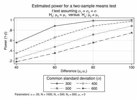
Finally, for our preferred sample size (500 per group), we calculate how standard deviations in calorie choice and effect sizes affect the statistical power.
Figure 3: Statistical power as a function of standard deviations and effect sizes. 3

2. Data Collection Procedures
The survey will be programmed and fielded using MMIC software (Multimode Interviewing Capability) on RAND’s American Life Panel (ALP). The 20 minute surveys will provide more data than a 30 minute or even longer survey on a newly recruited sample because baseline sociodemographics have been collected for this panel and we do no have to ask those questions. The ALP website can be found here: https://mmicdata.rand.org/alp/
Once OMB approval is received, RAND will program the final instrument for administration in the American Life Panel system using MMIC software and then pre-test it on a small sample of up to 100 participants from ALP. The pretest will be concluded within 8 weeks of OMB approval.
ALP creates an analytic data file to which RAND will merge relevant information from previous data collections, including demographics and variables like self-reported height and weight, using the MMIC data management system. While simple tests of means, possibly stratified by subgroups, would provide unbiased and internally valid results (it is an randomized experiments), our primary approach will be regression analysis to estimate how menu labeling affects calorie choices in different settings across different settings by sociodemographics. Additional statistical models may be used to analyze discrete choices, from standard economic models (such as multinomial or nested multinomial models) to models incorporating possible violations of classic economic models (e.g. attribute-non-attention).
Although national representativeness is not a requirement for the study question (differential effects to menu labeling by type of restaurant setting and sociodemographics), it enhances external validity. We do not plan to weight regression models, although we would use weights for descriptive statistics. As with all surveys based on random samples, the composition of the un-weighted sample will differ from the population composition. RAND constructs sampling weights to correct for this sampling error and to make a weighted sample representative of US population, benchmarking it against the Current Population Survey (CPS). This choice follows common practice in surveys of consumers, for example, the Health and Retirement Study (HRS). Raking was found to give the best results as it allows finer categorizations of variables of interest (in particular, age) than cell-based post-stratification does, while still matching these distributions exactly. Variables were created that account for interactions with gender or with the number of household members, as described below, so that distributions are matched separately for males and females, and for number of household members. Specifically, the following distributions are matched exactly is:
Gender x Age, with 10 Categories:
male, 18-32
male, 33-43
male, 44-54
male, 55-64
male, 65+
Categories (6)-(10) are the same as (1)-(5), except that they are for females instead of males.
Gender x age, with 10 categories: (1) male, 18-32; (2) male, 33-43; (3) male, 44-54; (4) male, 55-64; (5) male, 65+. Categories (6)-(10) are the same as (1)-(5), except that they are for females instead of males.
Gender x race/ethnicity, with 6 categories: (1) male, non-Hispanic white; (2) male, non-Hispanic African American; (3) male, Hispanic and other; (4) female, non-Hispanic white; (5) female, non-Hispanic African American; (6) female, Hispanic and other.
Gender x education, with six categories: (1) male, high school or less; (2) male, some college or associate's degree; (3) male, bachelor's degree or more; (4) female, high school or less; (5) female, some college or associate's degree; (6) female, bachelor's degree or more. All aggregate U.S. statistics for the SCPC were weighted using the sampling weights constructed in this manner.
Number of household members x (household) income, with twelve categories: (1) household with one individual, <$25,000; (2) household with one individual, $25,000-$49,999; (3) household with one individual, $50,000-$74,999; (4) household with one individual, $75,000+. Categories (5)-(8) are the same as (1)-(4), but for households with two individuals. Categories (9)-(12) are the same as (1)-(4), but for households with more than two individuals.
The Figures below show how the weighted ALP data compares to the US estimates from the CPS:
Figures

Figure
1: Comparison of weighted frequencies in ALP and CPS,
Males

Figure
2: Comparison of weighted frequencies in ALP and CPS, Females
Respondents of the survey are randomly assigned to different menus with and without calorie labeling. The primary goal is to estimate how calorie labeling differentially affect choices in different type of food outlets and consumers with different individual characteristics. Secondary goals are to estimate how consumers trade off prices and calories, and to calculate the welfare gains from labeling.
Each respondent will be presented with nine different menus (see list in Table 1). He/she will be asked to make food choices from each menu, followed by the final section of the survey where respondents will answer attitudinal and behavioral questions. The latter include questions about how hungry the respondent is at the time of the survey, how important characteristics like low price, value portions, and low calories are, and how much they generally pay attention to calorie and nutritional information.
Table 1: The 9 types of food outlets
Fast food burger chains |
Fast casual Asian restaurants |
Ice cream parlors |
Movie theatre snack bars |
Pizza-by-the-slice stands |
Organic, locally sourced restaurants |
Fast casual Mexican restaurants |
Salad/sandwich restaurants |
Coffee shops |
For each respondent, we will randomize the survey in the following ways:
1. For each individual the order of food outlets (fast food, Asian, ice cream, etc) will be randomly assigned. This will prevent any potential bias due to the order of appearance of the menus/food outlets.
2. For each food outlet the labeling of the menu shown is also randomly determined. This is the primary experiment, with the following treatments:
Treatment A: no calorie labels (this will serve as the “control”)
Treatment B: with calorie labels which meet the requirements of the FDA’s new regulation, i.e. the size of the calorie declaration must be no smaller than the size of the name or the price of the menu item it refers to, whichever is smaller. In general such calorie declarations must be in the same color, or a similar color as that used for the name of the associated menu item. The contextual statement about recommended daily caloric intake is shown. This is the “do minimum” treatment in which the new regulation will be met just barely.
Treatment C (for only four of the food outlets): We allow an alternative labeling design for the fast casual Asian restaurant, the salad/sandwich restaurant, the pizza-by-the-slice stand and the organic, locally sourced restaurant. The design will meet the requirements of the new regulation and use fonts that are more pronounced than Treatment B (e.g. through the use of a heavier font and/or colors that stands out from the background). While many restaurants will use minimal requirements, some are likely to feature calories more prominently (as Subway has done for a long time). This design will allow separating visibility from other restaurant effects (e.g. intentional health halo).
Because we have nine food outlets, five of them have two treatments (A and B), and four of them have three treatments (A to C), it is not possible to ensure that each individual will be shown equal numbers of Treatment A, B, and C. The extent that this may or may not introduce respondent bias will be determined empirically.
3. For some food outlets (fast-food burger, ice-cream, movie theatre, fast casual Mexican and coffee), the menus shown with have varying sets of prices. The options are:
Default prices
Lower calorie choices are approximately 20% cheaper (a “healthy dining subsidy”)
High calorie choices are approximately 20% more expensive (a “fat tax”).
This price manipulation breaks the perfect collinearity between prices and calories and allows the study team to estimate the price sensitivity and eventually the consumer gain from better choices.
For this data collection, we will target 2,000 completed responses of a 20 minute survey. Based on recent ALP surveys, we expect a 70% response rate. There have been over 430 surveys fielded using the ALP and the average response rate has been 70%. This is an average, so some surveys have done better and some worse, but we are expecting to get about 70%. Most surveys fielded to the ALP are about 20-25 minutes long and respondents are usually offered an incentive of $10-$20. Therefore, we believe our survey should fall within the average. The response rate does depend somewhat on how long the survey remains in the field and how many reminders are sent. We plan to field the survey for 2 to 4 weeks, depending on how quickly we reach our targeted response rate. Therefore, we will invite 2,850 individuals to participate in order to reach 2000 completes (we use reminders and incentives to achieve at least this response and also roll out samples in waves to assure our target completion rates). In previous ALP surveys, most individuals completing the interview respond within one week of the date the survey went into the field. In addition, through the MMIC system, we can send customized email reminders once per week for up to 4 weeks to panel members who have started the survey but not completed it and to those who have not started it. The reminders combined with the incentive are used to get to the 70% response rate.
4. Tests of Procedures or Methods
The RAND team has already heavily tested the survey to ensure the timing of the survey as well as to ensure that there are no problems with the MMIC programming of the tool or the wording of the questions. To test within the RAND team, we used eight graduate students from the Pardee RAND graduate school and did two focus groups with them. In each, the students were first instructed to go through the entire survey to test the length (average times were 21 minutes for the first group and 18 minutes for the second with no major outliers). Once that test was completed, two members of the RAND team lead discussions with the group to look at the wording of the questions and ensure that there was no confusion. The testers did not find any major problems with the survey. There were no extreme outliers in the timing either. These testers are likely to have more education than the average ALP member, so once OMB approval is received, the survey will be fielded to a small part of the sample (about 100 members of the ALP) as the first wave to ensure that there are no issues with the survey itself and that the timing remains at or below an average of 20 minutes per survey. However, the graduate student testers all regularly order food from the types of restaurants in the survey.
5. Statistical and Data Collection Consultants
The survey, sampling approach, and data collection procedures were designed by the RAND Corporation under the leadership of:
Roland Sturm, Ph.D.
RAND Corporation
1776 Main Street
Santa Monica, CA 90407
1 Code: power twomeans 0 , sd(350) power(0.8) diff (40 60 80 100) graph
2 power twomeans 0 , sd(200 400 600) power(0.8) diff (67) graph
3 power twomeans 0 , sd(300 400 500 600) n(1000) diff (40 60 80 100) graph
| File Type | application/vnd.openxmlformats-officedocument.wordprocessingml.document |
| File Modified | 0000-00-00 |
| File Created | 2021-01-24 |
© 2026 OMB.report | Privacy Policy