Attachment Y - Double Placement
Attachment Y - Diary Double Placement Report - September 2011.docx
Consumer Expenditure Surveys: Quarterly Interview and Diary
Attachment Y - Double Placement
OMB: 1220-0050
The Effect of Double Placements
on the Consumer Expenditure Diary Survey
By Sylvia A. Johnson-Herring, Susan L. King, Lucilla Tan, and Troy Olson
Introduction
Each household in the Consumer Expenditure (CE) Diary Survey is asked to record all of its expenditures over a 2-week period. The current policy calls for a field representative (FR) to visit each household in the sample three times. On the first visit the FR introduces herself, explains the survey, and leaves a CE-801 diary. All household members are asked to record their expenditures in the diary for a one-week period. On the second visit the FR collects the first week’s diary, answers any questions the respondents have, and leaves a second CE-801 diary. Again, all household members are asked to record their expenditures in the diary for a one-week period. On the third visit the FR collects the second diary, and the household is dropped from the survey and replaced by another household.
In certain situations FRs are allowed to leave two diaries on the first visit. In those situations the FR does not visit the household at the end of the first week, but collects the two diaries at the end of the second week, thus eliminating a visit and saving money. This report examines the differences between the single and double diary placement groups with respect to response rates, expenditures, demographic characteristics, and other measures of data quality.
Double placements do not appear to have any negative effects on the Diary Survey. Approximately 27% of eligible cases and 33% of completed diaries are currently double placed. If double placements were made at every household, the response rate would most likely remain at its current level or increase a few percentage points, to somewhere around 75%. Double placements are currently given more frequently to high-income households than to low-income households, which leads to double-placed diaries having higher reported expenditures than single-placed diaries. However, when the effects of income are controlled and expenditures are compared within income quintiles, double-placed diaries still have higher reported expenditures than single-placed diaries. Some of the differences are statistically significant, and some are not, but since double placements almost always produce higher reported expenditures, double placing diaries at every household would probably result in reported expenditures remaining at their current level or increasing a little.
Data
Response rates are calculated using CE Phase 2 Diary data from 2005 - 2010. Other analysis uses CE Phase 3 Diary data from 2005 - 2010. Phase 2 data has information on all eligible respondents including nonrespondents, whereas the Phase 3 data has information only on participating respondents.
DPLC_CHK is the variable on the Phase 2 and Phase 3 datasets that indicates whether a consumer unit (CU) received a double-placed diary. If the answer to the question “Was this a Week 1 and Week 2 double placement?” is “1” then the placement is a double placement. Otherwise DPLC_CHK is coded as “B” and it is considered to be a single placement. In this study, “1” is recoded as “YES” and “B” is recoded as “NO”.
METHODS and ANALYSIS
Double Placement Rates
For each year in the study period, 2005 – 2010, the number of single and double placements for both eligible cases and completed diaries are shown in Table 1. For most of the period the double placement rates hovered around 27% for eligible cases and 33% for completed diaries. They were lowest in 2005. In 2005 the option of double placing diaries was still relatively new (the option was first given in 2004), and it may have taken time for FRs to start double placing them or to start acknowledging a practice they were already doing. Figure 1 plots the double placement rate by year for eligible cases (CE Phase 2 Diary data) and completed diaries (CE Phase 3 Diary data).
Table 1. The number of single and double diary placements and rates of double placements for eligible cases and completed diaries (PICKCODE = 201 + 217) between 2005 and 2010
|
|
Eligible Cases |
|
Completed Diaries |
||||||
|
|
|
|
|
Double |
|
|
|
|
Double |
|
|
|
|
|
Placement |
|
|
|
|
Placement |
Year |
|
Single |
Double |
Total |
Rate (%) |
|
Single |
Double |
Total |
Rate (%) |
2005 |
|
16,454 |
4,855 |
21,309 |
22.78 |
|
10,867 |
4,259 |
15,126 |
28.16 |
2006 |
|
14,062 |
5,414 |
19,476 |
27.80 |
|
9,591 |
4,864 |
14,455 |
33.65 |
2007 |
|
13,969 |
5,636 |
19,605 |
28.75 |
|
8,891 |
4,856 |
13,747 |
35.32 |
2008 |
|
14,403 |
5,307 |
19,710 |
26.93 |
|
9,505 |
4,674 |
14,179 |
32.96 |
2009 |
|
14,408 |
5,616 |
20,024 |
28.05 |
|
9,612 |
5,011 |
14,623 |
34.27 |
2010 |
|
14,129 |
5,859 |
19,988 |
29.31 |
|
9,182 |
5,114 |
14,296 |
35.77 |
Total |
|
87,425 |
32,687 |
120,112 |
27.21 |
|
57,648 |
28,778 |
86,426 |
33.30 |
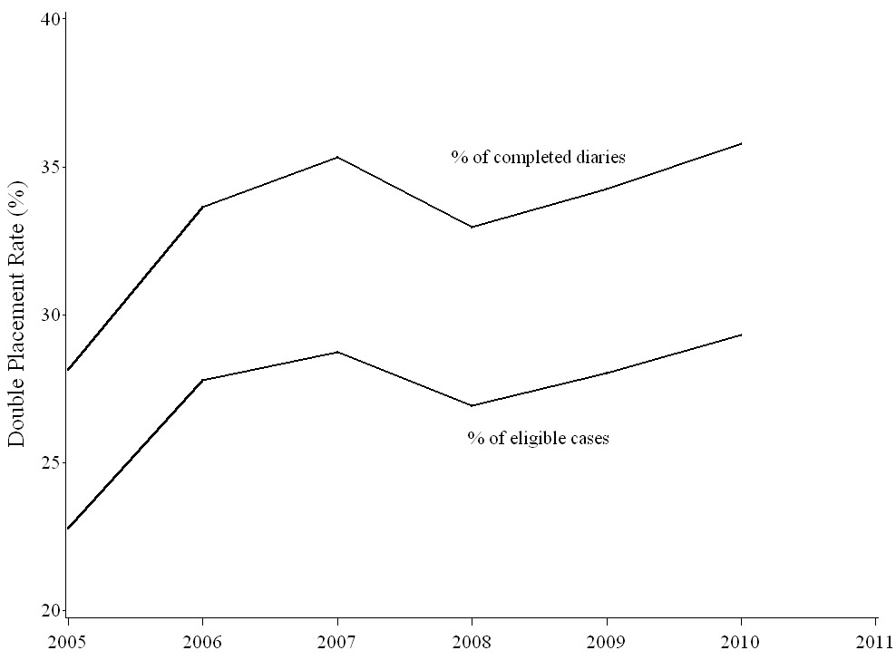
Figure 1. Percentage of eligible cases (Phase 2) and completed diaries (Phase 3) that were double placed from 2005-2010. Excluding 2005, the percentages are constant over time.
During the period 2005 – 2010, double placement rates varied by both region and regional office. Table 2 shows the variation by region. The highest double placement rate is in the Northeast, 45.45%, and the lowest double placement rate is in the South, 19.45%.
Table 2. Double placements by region for completed diaries
|
|
|
|
Double |
|
|
|
|
Placement |
Region |
Single |
Double |
Total |
Rate (%) |
Northeast |
9,116 |
7,596 |
16,712 |
45.45 |
Midwest |
12,271 |
9,113 |
21,384 |
42.62 |
South |
24,155 |
5,834 |
29,989 |
19.45 |
West |
12,106 |
6,235 |
18,341 |
33.99 |
Total |
57,648 |
28,778 |
86,426 |
33.30 |
Further investigation, Table 3, reveals that there is a significant variation in the frequency of double placements by regional office. Every regional office in the Northeast and Midwest has a double placement rate over 34%. Their double placement rates range from 34.19% in the Chicago regional office to 56.82% in the Detroit regional office. In the South and West, the double placement rates are variable. They range from 7.41% in the Dallas regional office to 55.70% in the Seattle regional office.
Table 3. Double placements by regional office for completed diaries
|
|
|
|
|
Double |
|
Regional |
|
|
|
Placement |
Region |
Office |
Single |
Double |
Total |
Rate (%) |
Northeast |
New York |
2,702 |
2,629 |
5,331 |
49.32 |
|
Boston |
3,085 |
2,704 |
5,789 |
46.71 |
|
Philadelphia |
4,474 |
2,973 |
7,447 |
39.92 |
Midwest |
|
|
|
|
|
|
Detroit |
2,986 |
3,930 |
6,916 |
56.82 |
|
Kansas City |
2,644 |
1,506 |
4,150 |
36.29 |
|
Chicago |
5,962 |
3,098 |
9,060 |
34.19 |
|
|
|
|
|
|
South |
Atlanta |
6,039 |
2,612 |
8,651 |
30.19 |
|
Charlotte |
8,199 |
1,780 |
9,979 |
17.84 |
|
Dallas |
8,165 |
653 |
8,818 |
7.41 |
|
|
|
|
|
|
West |
Seattle |
3,080 |
3,873 |
6,953 |
55.70 |
|
Denver |
4,149 |
2,216 |
6,365 |
34.82 |
|
Los Angeles |
6,163 |
804 |
6,967 |
11.54 |
Total |
|
57,648 |
28,778 |
86,426 |
33.30 |
Why Do Double Placements Occur?
There are three questions to be investigated in this and later sections: (1) Do regional office policies vary on double placements? (2) Who initiates the request for double placements, the field representative or the respondent? and (3) Are single and double diary respondents different?
There are two variables that are especially valuable in answering the first two questions, DPLCRES and DPLCSPC. The variable DPLCRES has a list of coded reasons for the FR to select from when making a double placement, and the variable DPLCSPC gives a space for the FR to write a brief verbal explanation. When double placing a diary, FRs select one of the coded reasons in Table 4 to explain their decision.
Table 4. Reasons and percentages for phase 3 diary double placement (DPLCRES)
Reason for Double Placement |
2005 |
2006 |
2007 |
2008 |
2009 |
2010 |
No one available for Week 1 pickup |
51.58% |
50.82% |
49.49% |
51.22% |
35.68% |
37.33% |
CU requests no Week 1 pickup |
33.81% |
35.30% |
37.13% |
34.32% |
33.77% |
32.68% |
FR does not work on Sunday |
1.10% |
1.03% |
0.99% |
1.28% |
1.76% |
1.58% |
Traveled more than 50 miles to place Diary |
--- |
--- |
--- |
--- |
15.59% |
16.93% |
Other |
13.50% |
12.85% |
12.40% |
13.18% |
13.21% |
11.48% |
This table shows the decision to double place diaries is made jointly by FRs and respondents, with more of the decision probably being made by the respondents. The reason “Traveled more than 50 miles to place Diary,” was added in 2009. Based on the 2009 and 2010 percentages, it appears that the extreme travel distances required by FRs was included in the category “No one available for Week 1 pickup” in prior years. Interpreting the data for “No one available for Week 1 pickup” is a little difficult because its meaning is not clear – is it the respondent or the FR who is not available for week 1 pickup?
Another variable, DPLCSPC, provides a space for FRs to give a brief explanation of the reason for the double placement. These comments shed further light on the questions about varying regional office policies towards double placements, and who initiates the request for double placement, the FRs or the respondents? FRs wrote over 2,800 comments in this field in 2005 – 2010, with more than 100 of them saying things such as: “RO policy”; “RO protocol”; “RO directive”; and “RO said to double place.” These comments lend support to a difference in regional office policies on double placements. The other comments said things such as: “FR out of town next week”; “FR will be in RO for training”; “Respondent won’t be home”; and “Respondent having surgery.” These other comments suggest the reasons for double placing diaries come equally from the FRs and the respondents.
To further investigate the source of double placements, a search of the data base was conducted on 81 collected variables to measure their association with double placements. The goal was to examine as many variables as possible and use Pearson’s chi-square test of independence to rank the variables. Since many of the p-values were beyond SAS’s computational capability, the chi-square statistic was transformed into a z-score using the “Wilson-Hilferty transformation.” The transformation allows a two-dimensional chi-square statistic (chi-square score plus degrees of freedom) to be converted into a one dimensional z-score, allowing the variables to be ranked according to their degree of statistical significance. See Appendix A for more details, SAS Code, and complete listing of potential explanatory variables examined and their z-scores. The top ten explanatory variables are listed below in Table 5.
Table 5. Top ten explanatory variables
Ranking |
Variable |
Definition |
Z-Score |
1 |
FIELD_REP2 |
Last FR to touch the case |
154.84 |
2 |
FIELD_REP1 |
First FR to touch the case |
152.31 |
3 |
PSU |
2000 Sample Design PSU |
99.31 |
4 |
FIELD_REP3 |
First SFR to touch the case |
91.17 |
5 |
FIELD_REP4 |
Last SFR to touch the case |
91.10 |
6 |
NUMVISIT |
Number of visits made to collect data |
67.72 |
7 |
REG_OFF |
Census Regional Office |
60.83 |
8 |
CBSASIZE |
Population size of CBSA |
44.16 |
9 |
OUTCOME |
Diary Outcome Code for both weeks (final outcome code) |
42.07 |
10 |
DESCRIP |
Housing Unit Type |
39.40 |
Variables with higher z-scores indicate a stronger correlation with double placements. Based on the results in Table 5, FRs play an important role in the decision to double place diaries. Of the first six variables in the table, only PSU is not controlled by the FR. OUTCOME is under the control of both the FR and the respondent.
Previously, the difference in double placement rates among regions and regional offices was noted (Tables 2 and 3), and comments in the DPLCSPC field suggested that policies on double placements may differ by regional office. On the table above REG_OFF is the seventh best explanatory variable, which supports this hypothesis, and REGION is the eleventh best explanatory variable. Additional geographic variables in the top ten explanatory variables are PSU and CBSASIZE.
Other variables on the list are NUMVISIT and DESCRIP. The variable NUMVISIT is the number of visits made to collect the data. Double placements exceed single placements only on the second visit. DESCRIP describes the type of housing unit, e.g., house, apartment, group quarters, or mobile home.
The third question addressed in this section is: “Are single and double diary respondents different?” Socio-demographic variables are useful in addressing this question. This question is important because if the two groups are different, then predictions of response rates and expenditures if all diaries are double placed will be affected. Of all the socio-demographic variables examined, tenure has the highest z-score and is ranked thirteenth. Other socio-demographic variables, such as language spoken, household size, and gender of the reference person, have smaller z-scores and are ranked lower. Overall, the z-scores of socio-demographic variables indicate differences between single and double diary respondents, but the differences are less important than variables related to FRs, regional offices, number of contact attempts, etc. in the decision to double place diaries.
In conclusion, the evidence indicates that there are varying regional office policies on double placements; single and double diary respondents have different socio-demographic characteristics; and the decision to double place diaries is made jointly by FRs and respondents. However, it is not clear whether the FRs or respondents drive the decision process, since Table 4 indicates that respondents tend to drive the decision process, while Table 5 indicates that FRs tend to drive it.
Do Double Placements Affect Response Rates?
Response rates are the ratio of completed diaries to eligible cases and are multiplied by 100%. Completed diaries include CUs who are temporarily absent. Eligible cases include completed diaries plus Type A nonrespondents. Thus,
 .
.
Tables 6.1, 6.2, and 6.3 show the annual response rates for all eligible cases, for eligible cases with single-placed diaries, and for eligible cases with double-placed diaries, respectively.
Table 6.1 CE diary annual response rates
Collection |
Completed |
Eligible |
Response |
Year |
Interviews |
Cases |
Rate |
2005 |
15,126 |
21,309 |
70.98% |
2006 |
14,455 |
19,476 |
74.22% |
2007 |
13,747 |
19,595 |
70.14% |
2008 |
14,179 |
19,710 |
71.94% |
2009 |
14,623 |
20,024 |
73.03% |
2010 |
14,296 |
19,988 |
71.52% |
Table 6.2 CE annual response rates for single-placed diaries
Collection |
Completed |
Eligible |
Response |
Year |
Interviews |
Cases |
Rate |
2005 |
10,867 |
16,454 |
66.04 |
2006 |
9,591 |
14,062 |
68.21 |
2007 |
8,891 |
13,963 |
63.65 |
2008 |
9,505 |
14,403 |
65.99 |
2009 |
9,612 |
14,408 |
66.71 |
2010 |
9182 |
14,129 |
64.99 |
Table 6.3 CE annual response rates for double-placed diaries
Collection |
Completed |
Eligible |
Response |
Year |
Interviews |
Cases |
Rate |
2005 |
4,259 |
4,855 |
87.72 |
2006 |
4,864 |
5,414 |
89.84 |
2007 |
4,856 |
5,632 |
86.16 |
2008 |
4,674 |
5,307 |
88.07 |
2009 |
5,011 |
5,616 |
89.23 |
2010 |
5,114 |
5,859 |
87.28 |
Tables 6.1, 6.2, and 6.3 show response rates being considerably higher for CUs given double placements than for CUs given single placements. The response rate for CUs given double placements is around 88%, while the response rate for CUs given single placements is around 66%.
Before jumping to the conclusion that double placements can increase CE’s response rate to 88%, a note of caution must be given. First, no controls were placed on the CUs that were offered each type of placement. If the two sets of CUs have different characteristics, then the differences in response rates may be due to their different characteristics rather than the different type of placement. In the next section it will be shown that their characteristics are indeed different. Furthermore, it is not clear how or when FRs decide to check the “double placement” box on their CAPI instruments. It is possible that they check the box only after successfully double placing two diaries, leaving the box unchecked in all other situations – single placements, refusals, noncontacts, etc. If this is true, then the response rates in Tables 6.1, 6.2, and 6.3 will contain significant biases, with the response rates of single-placed diaries being under-estimated and the response rates of double-placed diaries being over-estimated. Thus a better way of examining response rates may be the plot shown in Figure 2.
Figure 2 plots response rates versus double placement rates and overlays a regression line. Each dot represents a PSU summary for one of the five years in the study. The regression line is:
Response rate = 71.71 + 0.05 × double placement rate
Using this equation, increasing the double placement rate from its current level of 33% to 100% would increase the Diary Survey’s response rate from 73% to 77%. In other words, if the CE program changed its double placement policy and double placed all diaries, the response rate would increase by four percentage points. This seems more plausible than the results indicated in Tables 6.1, 6.2, and 6.3.
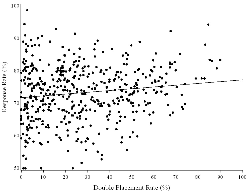
Figure 2. Response rates are plotted against double placement rates. Each point represents a PSU for one of the five study years, and the regression line is overlayed on the graph. The regression line is slightly positive as indicated by the small slope, 0.05. This says as double placements increase, the response rate will slightly increase.
Are Single and Double Diary Respondents Different?
The third question is: “Are single and double diary respondents different?” If there are differences between the two groups, it may have implications regarding response rates and expenditure estimates if all CUs were given a double diary. In this section, the socio-demographic differences between single and double diary placement CUs are explored. These comparisons are based on respondents. Comparisons based on non-respondents are not feasible because relatively little information is known about them.
QUINTILE is a categorical variable created from the weighted cumulative percent ranking of total income. CUs in the CE database are sorted by their income, from poor to rich, after which they are assigned to an income quintile. Each 20% increment is a quintile. Those in the lowest 20% are put in the first quintile, and those in the highest 20% are put in the fifth quintile. Figure 3 shows the percent of double placements (black) versus single placements (gray) for each income quintile. This graph shows that the frequency of double placements increases with income.
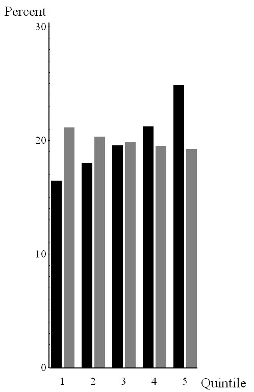
Figure 3. Each black bar shows the percentage of double-placed diaries that are in each of the five income quintiles. Similarly, each gray bar shows the percentage of single-placed diaries that are in each of the five income quintiles. As the graph shows, the frequency of double placements increases directly with income, while the frequency of single placements decreases slightly with income.
CUTENURE is a categorical variable describing a CU’s housing tenure. It has six categories:
1 Owned with mortgage
2 Owned without mortgage
3 Owned- mortgage status not reported
4 Rented
5 Occupied without payment of cash rent
6 Student housing
This variable shows double placements (black) are more common than single placements (gray) for owners with and without mortgages. Single placements are more common for renters.
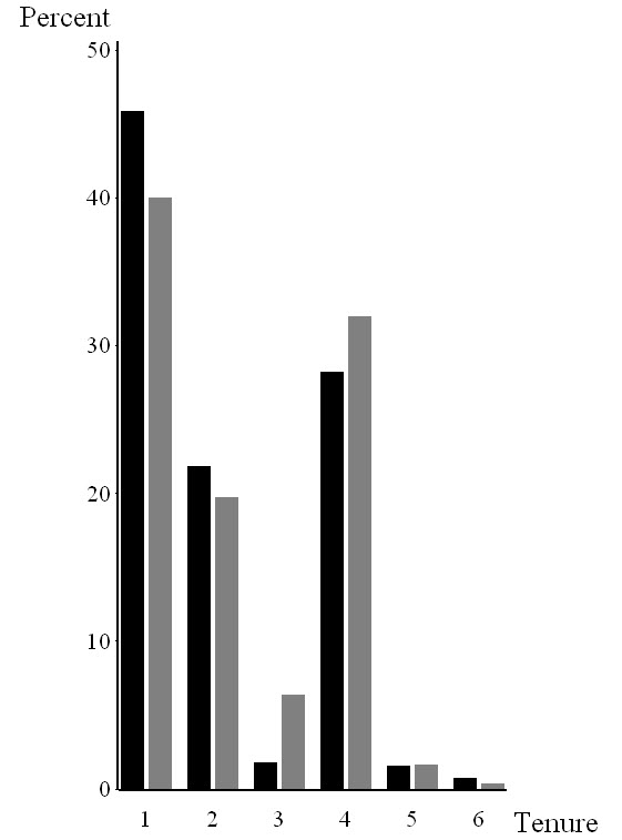
Figure 4. Double placements are more common for homeowners than for renters.
EDUC_REF is a categorical variable describing the educational attainment of a CU’s reference person. It has nine categories:
00 Never attended
10 1st – 8th grade
11 9th – 12th grade – no high school diploma
12 High school graduate
13 Some college – no degree
14 Associates degree
15 Bachelors degree
16 Master’s degree
17 Professional/Doctorate degree
This variable shows double placements (black) are more common than single placements (gray) for CUs whose reference person has an associate’s degree or higher. Single placements are more common for CUs whose reference person has less education.
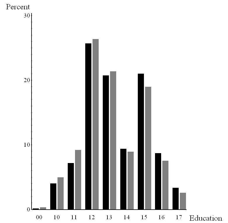
Figure 5. Double placements are more common for CUs whose reference person has an associate’s degree or higher than for CUs whose reference person has less than an associate’s degree.
AGE_REF is a categorical variable describing the age of the CU’s reference person. In this report it was collapsed into ten-year increments (<20, 20-29, 30-39, 40-49, etc.). This variable shows double placements (black) are more common than single placements (gray) for CUs whose reference person is middle aged (in their 40’s and 50’s). Single placements are more common for other age groups.
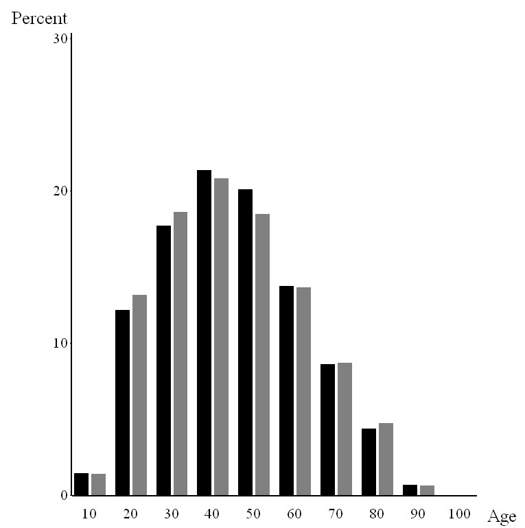
Figure 6. Double placements are more common for CUs whose reference person is in their 40’s and 50’s than for CUs whose reference person is younger or older than that.
REF_RACE is a categorical variable describing the race of a CU’s reference person. The categories are:
1 White
2 Black
3 Other (Native American, Asian, Pacific Islander, and Multi-race)
This variable shows double placements (black) are more common than single placements (gray) for CUs whose reference person is white. Single placements are more common for all other CUs.
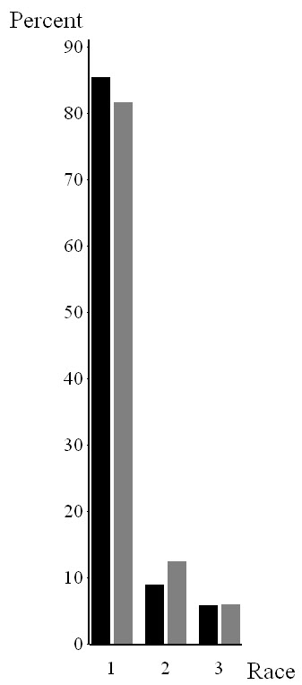
Figure 7. Double placements are more common for CUs whose reference person is white than for CUs whose reference person in non-white.
FAM_TYPE is a categorical variable describing the size of a CU, the age of the CU members, and the relationship between the CU members. It has nine categories:
1 Husband and wife only
2 Husband and wife with their oldest child under 6 years
3 Husband and wife with their oldest child between 6 and 17 years
4 Husband and wife with their oldest child over 17 years
5 All other husband and wife families
6 One male parent with at least one child under 18
7 One female parent with at least one child under 18
8 Single consumers
9 Other families
This variable shows double placements (black) are more common than single placements (gray) for husband-and-wife families in the first four categories. Single placements are more common for all other categories.
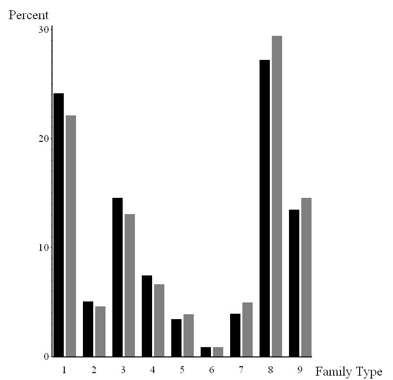
Figure 8. Double placements are more common for husband-and-wife families than for other types of families.
FAM_SIZE is a categorical variable describing the number of people in a CU. In this report it was collapsed into six values (1, 2, 3, 4, 5, 6+). This variable shows double placements (black) are more common than single placements (gray) for CUs with 2 – 4 people. Single placements are more common for all other CUs. However, there is not a large difference between them.
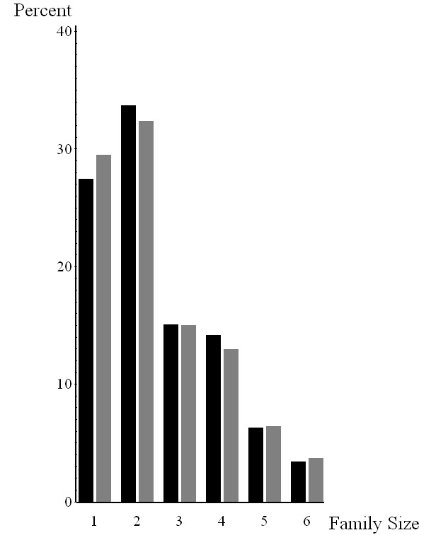
Figure 9. Double placements are more common for CUs having 2 – 4 people than for other CUs.
URBAN is a categorical variable describing the population density of the area in which a CU lives. It has two categories:
1 Urban
2 Rural
This variable shows double placements (black) are more common than single placements (gray) for CUs living in rural areas. However, the difference is small.
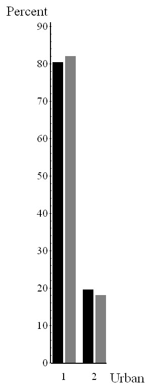
Figure 10. Double placements are slightly more common for CUs living in rural areas than for CUs living in urban areas.
The final variable to be examined is STRATUM. The U.S. Census Bureau orders all of the households on its sampling frame from poor to rich prior to drawing a systematic sample of them. The purpose is to make sure every economic segment of the American population is well-represented in the CE survey. The ordering is done with the variable STRATUM, which is based on household tenure, income, and CU size. Table 7 shows the ordering. Renters in the lowest income quartile are at the poor end of the scale, and homeowners in the highest income quartile are at the rich end. The orange arrows show the ordering.
All stratification codes are shown in black or gray. If the majority of diaries are double placed then the stratification code is black. If the majority of diaries are single placed then the stratification code is gray. Based on this coloring scheme, a pattern can be seen in Table 7 in which single placements dominate in the poorest CUs (i.e., renters in the two lowest income quartiles), while double placements dominate in the wealthiest CUs (i.e., owners in the highest two income quartiles).
The magnitude of the single and double placement rates for each value of STRATUM can be seen in Figure 11. Stratum 42 has the largest difference favoring single placements over double placements (5.03% versus 4.29%), while stratum 81 has the largest difference favoring double placements over single placements (4.56% versus 4.01%). In general, there are more double placements in smaller CUs (1 and 2 persons) than in the larger CUs (3 and 4+ people). New construction is coded as blank or “B” and represents 9.28% of the diaries.
Table 7. CE Stratification Code Sort Order
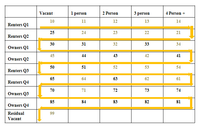
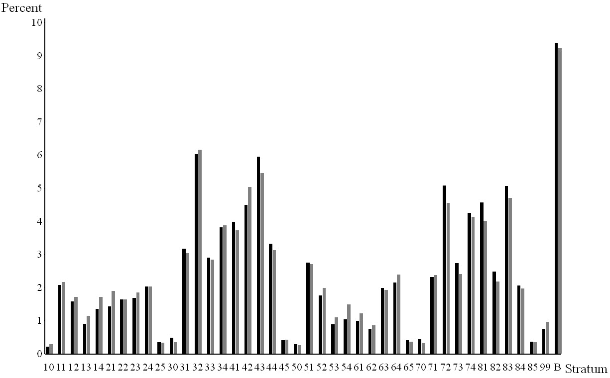
Figure 11. Double diary placements are in black and single diary placements are in gray. The graph shows the magnitude of the differences between double and single diary placements by stratum.
In conclusion, the socio-demographic data shows that diaries are not double placed at random. Although diaries are double placed in every segment of the population, there is a difference between the households given single and double placements. Double placements occur more frequently in CUs that have a high income, own their own home, have a high level of education, are middle aged, are white, and are a small husband-and-wife family.
Are Double Placement Data Falsified?
Double placements are only supposed to be made in rare situations, so it seems natural to wonder whether FRs who violate this basic principle by double placing diaries often also violate other rules. Therefore it was decided to test the data for evidence of falsification. There are four ways to falsify the data: invent expenditure data for a CU (curbstoning); code the address of an occupied housing unit as Type B (housing unit is unoccupied); code the address as Type C (no housing unit at the assigned address); or code the CU as temporarily absent (PICKCODE=217). All of these are ways FRs can avoid being penalized for Type A nonresponses, not getting an interview at an occupied housing unit. We did not test the data for curbstoning. Of the other three methods of falsification, the third is the least likely to occur because there is little incentive for FRs to falsify the response in that way. BLS considers temporarily absent CUs to be “good” interviews, but the U.S. Census Bureau, the FRs’ employer, considers them to be Type B nonresponses.
A series of graphs are presented below that test for data falsification. Due to small sample sizes it is not feasible to represent each FR on the graph. In 2010, one-third of the FRs collected fewer than 20 diaries. Therefore, the data is summarized to the PSU level for each year.
In Figure 12, the rate of ineligible housing units (Type B and Type C) is plotted against the double placement rate. The linear regression line is overlayed on the scatter plot. As the double placement rate increases, the linear regression line remains constant, indicating that FRs who double place diaries are not falsifying the data.
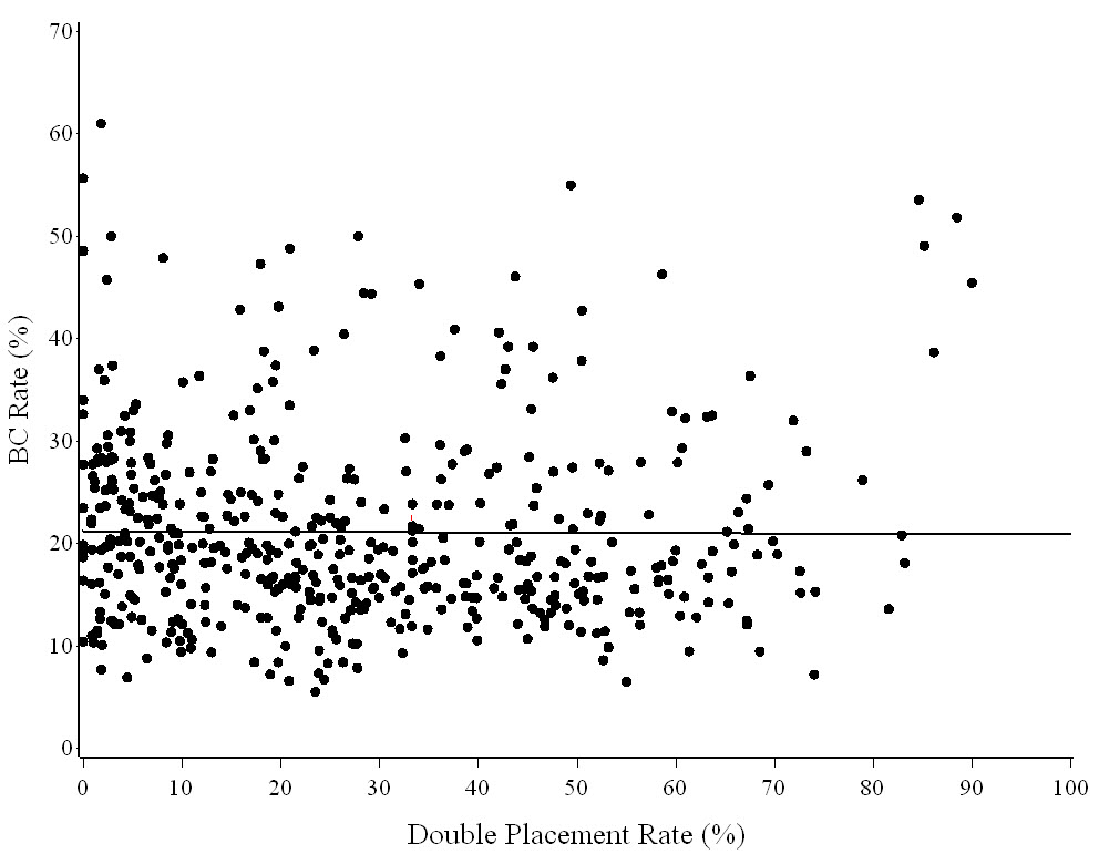
Figure 12. The rate of ineligible housing units is plotted against the double placement rate. The linear regression line is constant, indicating that FRs are not falsely reporting housing units to be unoccupied or nonexistent.
In Figure 13, the rate of temporarily absent CUs is plotted against the double placement rate. The overlayed regression line is decreasing as the double placement rate increases. Low temporarily absent rates are considered to be good, so this indicates that FRs who double place diaries are not falsifying the data.
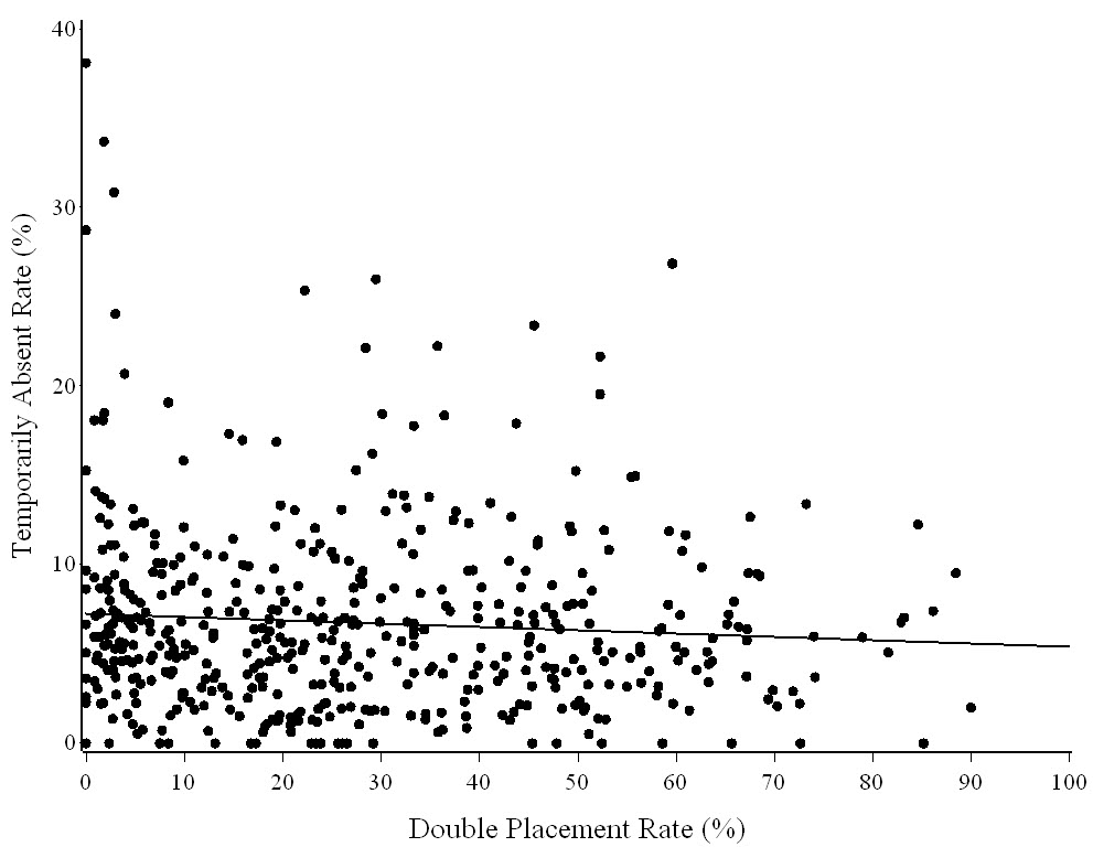
Figure 13. The rate of temporarily absent CUs is plotted against the double placement rate. The linear regression line is decreasing as double placements increase, indicating that FRs are not falsely reporting CUs to be temporarily absent.
In Figure 14, the average interview length is plotted against the double placement rate. The black dots and the black regression line indicate the average interview length for double-placed diaries, while the gray dots and the gray regression line indicate the average interview length for single-placed diaries. In general, the average interview length is longer for double-placed diaries. Longer interviews are considered to be good, and the slope of the black regression line is increasing as the double placement rate increases, which indicates longer interviews for double-placed diaries. This suggests the FRs who double place diaries are not falsifying the data.
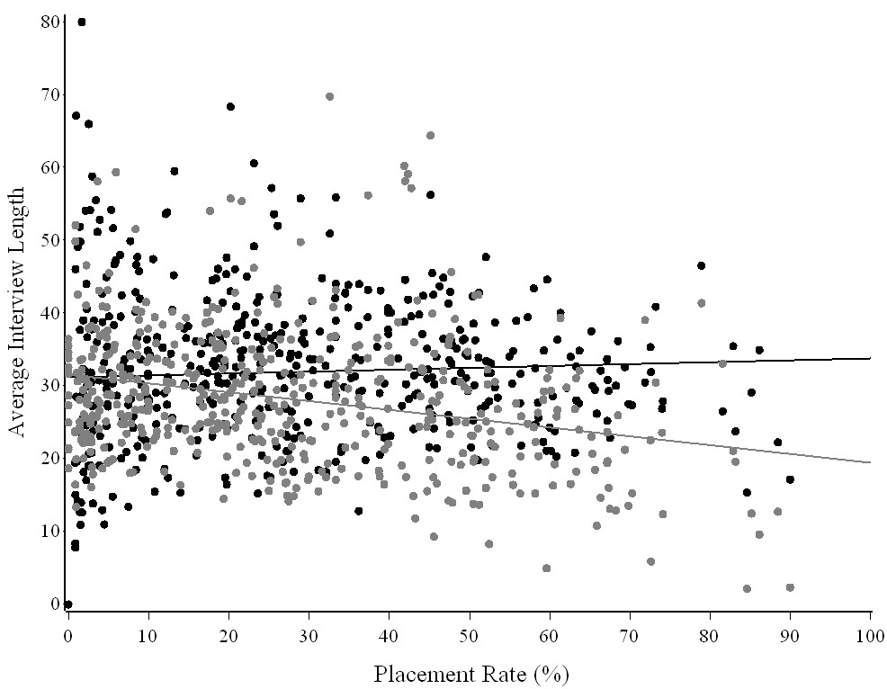
Figure 14. The black dots indicate the average interview length for double-placed diaries, and the gray dots indicate the average interview length for single-placed diaries. As indicated by the regression lines, the average interview length is longer for double-placed diaries, suggesting that FRs are not falsifying the data.
There are three modes of data collection: personal visit, telephone interview, and not recorded. Personal visits outnumber both telephone interviews and not recorded. Figure 15 shows that the percent of diaries collected by personal visits remains constant at 70% as double placements increase. Personal visits are considered to be good. This indicates that the FRs who double place diaries are not falsifying the data. The percent of telephone interviews increases and the percentage of not recorded mode of data collection decreases as double placements increase.
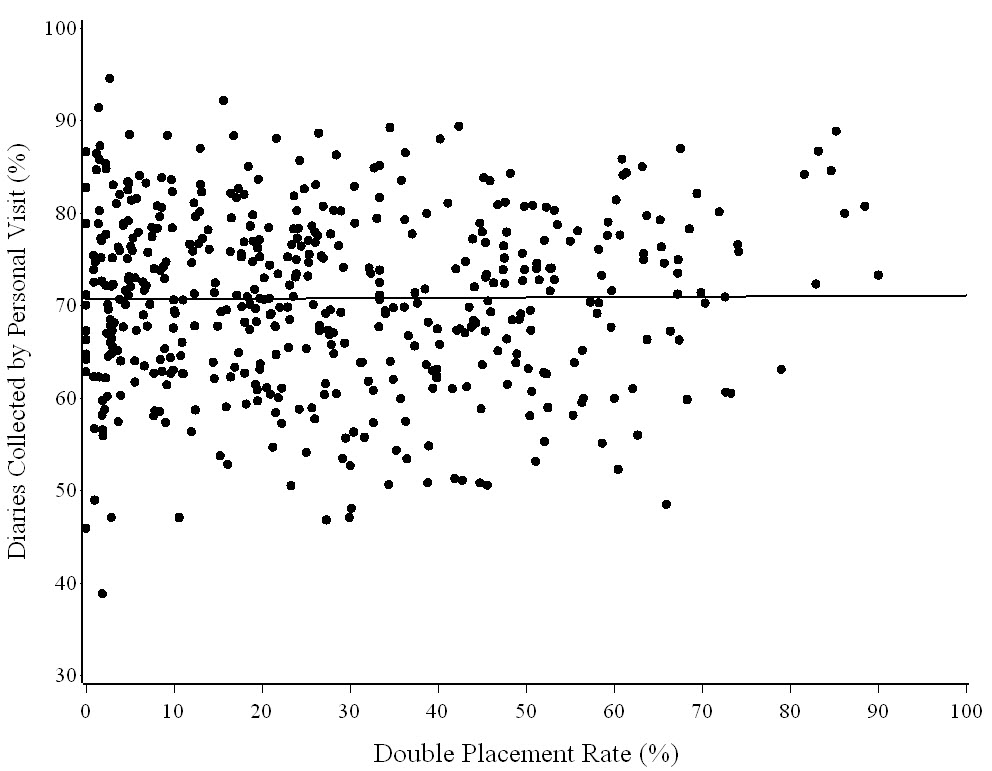
Figure 15. The percentage of personal visits is plotted against the double placement rate. The overlayed regression line is constant at 70%, indicating that the FRs are not falsifying the data.
In conclusion, all four graphs (Figures 12 - 15) indicate that FRs who double place diaries are honest and are not falsifying the data.
Do the Expenditures in Single and Double Placed Diaries Differ?
Total expenditures of a CU (ZTOTAL) are available in Phase 3 beginning in 2007. Therefore, expenditures from 2007 - 2010 are used to investigate whether there is a difference in expenditures between single and double placements for completed diaries. Completed diaries include CUs who are temporarily absent and those who did not have any expenditures for a week. Table 8.1 shows the mean weekly expenditures by income quintile for all completed diaries (PICKCODE=201 + 217). Table 8.2 shows the mean weekly expenditures for all completed diaries of CUs who were at home and not temporarily absent (PICKCODE=201). Finally, Table 8.3 shows statistics for temporarily absent CUs.
Table 8.1. Mean expenditures and statistics for all potential diaries (PICKCODE=201 + 217) by income quintile
|
|
|
|
Mean Weekly Expenditures |
|
|
|
|
Double |
Single |
Double |
Double Placed |
Single Placed |
|
|
|
Placed |
Placed |
Placed |
Diaries + 95% |
Diaries + 95% |
|
|
Quintile |
Diaries |
Diaries |
Diaries (%) |
CI ($) |
CI ($) |
t-test |
p-value |
1 |
3,259 |
7,862 |
29.30 |
392.13 ± 28.73 |
326.50 ± 24.14 |
3.43 |
0.000632 |
2 |
3,519 |
7,528 |
31.85 |
529.50 ± 34.12 |
485.92 ± 46.44 |
1.48 |
0.138600 |
3 |
3,800 |
7,386 |
33.97 |
689.31 ± 41.86 |
595.84 ± 31.03 |
3.53 |
0.000458 |
4 |
4,130 |
7,267 |
36.24 |
902.40 ± 50.65 |
814.42 ± 60.16 |
2.19 |
0.028595 |
5 |
4,947 |
7,147 |
40.90 |
1,373.74 ± 97.71 |
1,322.97 ± 76.12 |
0.80 |
0.421920 |
Total |
19,655 |
37,190 |
34.58 |
815.63 ± 33.82 |
689.27 ± 36.18 |
5.00 |
0.000001 |
Table 8.2. Mean expenditures and statistics for all completed diaries (PICKCODE=201) by income quintile
|
|
|
|
Mean Weekly Expenditures |
|
|
|
|
Double |
Single |
Double |
Double Placed |
Single Placed |
|
|
|
Placed |
Placed |
Placed |
Diaries + 95% |
Diaries + 95% |
|
|
Quintile |
Diaries |
Diaries |
Diaries (%) |
CI ($) |
CI ($) |
t-test |
p-value |
1 |
3,221 |
6,758 |
32.28 |
396.20 ± 29.52 |
379.10 ± 28.03 |
0.82 |
0.410780 |
2 |
3,469 |
6,421 |
35.08 |
537.50 ± 34.48 |
565.90 ± 50.81 |
-0.91 |
0.362800 |
3 |
3,765 |
6,501 |
36.67 |
695.70 ± 42.02 |
673.67 ± 34.73 |
0.79 |
0.428460 |
4 |
4,102 |
6,685 |
38.03 |
908.51 ± 50.19 |
884.30 ± 33.23 |
0.57 |
0.571370 |
5 |
4,935 |
6,930 |
41.59 |
1,376.63 ± 97.13 |
1,364.42 ± 79.11 |
0.19 |
0.848970 |
Total |
19,492 |
33,295 |
36.93 |
822.33 ± 33.65 |
768.718 ± 39.55 |
2.02 |
0.043279 |
Table 8.3. Statistics for temporarily absent CUs
|
Double |
Single |
|
Percent of Temporarily |
|
Placed |
Placed |
Total |
Absent CUs that were |
Quintile |
Diaries |
Diaries |
Diaries |
Double Placed |
1 |
38 |
1,104 |
1,142 |
3.33% |
2 |
50 |
1,107 |
1,157 |
4.32% |
3 |
35 |
885 |
920 |
3.80% |
4 |
28 |
582 |
610 |
4.59% |
5 |
12 |
217 |
229 |
5.24% |
Total |
163 |
3,895 |
4,058 |
4.02% |
The first observation from Tables 8.1 and 8.2 is that the percent of double-placed diaries increases as income increases. They increase from approximately 30% of all completed diaries in the lowest income quintile to 40% of all completed diaries in the highest income quintile. This means the data in the bottom row, where all five income quintiles are combined, is a little misleading because the column for double-placed diaries has more wealthy CUs and fewer poor CUs than the column for single-placed diaries. Thus the t-tests in the last row of Tables 8.1 and 8.2 give results that appear to be more significant than they really are.
The second observation is that the number of temporarily absent CUs decreases as income increases. They decrease from approximately 10% of all completed diaries in the lowest income quintile to 2% of all completed diaries in the highest income quintile. Since the expenditures of temporarily absent CUs are defined to be zero dollars, the mean expenditures in the bottom row of Table 8.1, where all five income quintiles are combined, may give too much weight to wealthy CUs and too little weight to poor CUs. Thus the mean expenditures in the bottom row of Table 8.1 may be a little low.
The third observation is that Table 8.3 shows the distribution of temporarily absent CUs between the single and double placement groups is the same across income quintiles. Approximately 96% of the temporarily absent CUs are single placements, and 4% of them are double placements, and these proportions are the same in all five income quintiles. Since the expenditures of temporarily absent CUs are defined to be zero dollars, this lopsided assignment of CUs to the two placement groups suggests that the expenditures of CUs with single-placed diaries in Table 8.1 may be under-estimated relative to those with double-placed diaries. Thus the t-tests in all of the individual income quintiles of Table 8.1 may give results that appear to be more significant than they really are.
The problems caused by these three observations leave us with the five individual income quintiles in Table 8.2. Four out of five of them show the mean weekly expenditure being higher in double-placed diaries than in single-placed diaries, but none of the differences are statistically significant. As a result, based on the information currently available, it seems reasonable to conclude that double placing diaries at all households would probably result in reported expenditures either remaining at their current level or increasing a little.
TRANSPORTATION SAVINGS
Data from four recent quarters were used to estimate transportation cost savings. Assuming the cost per mile is $0.505, the travel cost saving from switching to complete double placement over the current placement mixture is approximately $170,000. The table in Appendix B provides further details on the estimation of transportation cost. All three classes of respondents, Type A, Type B, and Type C were included in the analysis. Personnel cost savings from switching to double diary placements are more significant in terms of dollars but are more difficult to estimate. These savings would be smaller than a 1/3 reduction in hours and salary and benefits.
DATA QUALITY
The frequency of double and single diary placements was compared for several of the Phase 3 data edits using quarter data from 2008 – 2009. The comparison tables for significant imputed and other edited variables are given in Appendix C. In summary, no significant data quality issues arose due to double diary placement.
CONCLUSION
FRs have been double placing diaries for a long time. In 2004 CE management decided to acknowledge the practice and establish guidelines for when it can be done. This report examined various aspects of double placements during the period 2005 – 2010 to determine what effect it has on the Diary survey’s data. Overall, double placements do not appear to have any negative effects on the Diary survey. Here is a summary of specific findings from this report:
Approximately 27% of all eligible cases and 33% of all completed diaries are currently double placed.
Double placement rates vary by regional office and by region of the country. Double placement rates vary from 7.41% of completed diaries in the Dallas regional office to 56.82% of completed diaries in the Detroit regional office. This is strong evidence of varying regional office policies on double placements. Double placement rates also vary by region of the country, indicating that respondents have different attitudes about double placements depending on their geographic location, but the evidence for this is much weaker.
The decision to double place diaries is made jointly by FRs and respondents, but it is not clear who drives the decision process more. Table 4 indicates the decision is driven by respondents, while Table 5 indicates it is driven by FRs.
FRs who double place diaries frequently are just as honest as FRs who double place them infrequently. There is no evidence of data falsification by either group of FRs. Type A,B,C nonresponse rates as well as the temporarily absent rate are the same for both groups of FRs.
Households that are given single and double placements have different socio-demographic characteristics. Households that are given double placements tend to be wealthy, well-educated, white, middle-aged, homeowners, husband-and-wife families, and who speak English. These are characteristics that are typically associated high survey response rates, and it may be part of the reason that households given double placements have higher response rates than those given single placements. These characteristics are also associated with high expenditures, and it may be part of the reason that households given double placements have higher expenditures than those given single placements.
Double placements do not have any negative effects on the response rate. The Diary survey’s response rate is currently in the 70% - 75% range. If double placements were made at every household, the response rate would most likely remain at its current level or increase a few percentage points, to somewhere around 75%.
Double placements do not have any negative effects on the reported expenditures. Comparisons of mean weekly reported expenditures by income quintile (PICKCODE=201 only) show that households with double-placed diaries reported more expenditures than those with single-placed diaries in four of the five income quintiles. Not one of the differences wwas statistically significant, but taken together they suggest double placing diaries at every household would probably either leave the reported expenditures unchanged or increase them a little.
Switching from the current 27% double placement rate to a 100% double placement rate would reduce FR travel costs by 25% - 30%. The travel cost for the Diary survey is currently around $610,000 per year. If diaries were double placed at every household, travel costs would decrease by $170,000 per year to approximately $440,000. Note: These figures only represent mileage costs. They do not include salary costs. The savings from salaries may be significantly greater.
Overall, double placements do not appear to have any negative effects on the Diary survey. If diaries were double placed at every household, the survey’s response rate and the reported expenditures would probably either remain at their current levels or increase a little, while FR travel costs would decrease by about $170,000 per year.
Appendices
Appendix A: Program, Background Information, and Results for Variables Associated with Double Placement
SAS Program Used to Search for Variables Associated with Double Placements
The program below was used to search the Diary database for variables associated with double placements. The basic idea was to examine as many variables as possible and perform a chi-square test of independence. The variables that failed the chi-square test of independence were considered to be associated with double placement.
The following is an example using the language spoken in a household and the day of the week the FR drops off the diaries:
|
Double Placement? |
|
|
Diary Placement |
Double Placement? |
|
||
Language |
Yes |
No |
Total |
|
Day |
Yes |
No |
Total |
1 (English) |
22,814 |
41,654 |
64,468 |
|
Sunday |
2,359 |
4,611 |
6,970 |
2 (Spanish) |
402 |
2,084 |
2,486 |
|
Monday |
3,940 |
7,832 |
11,772 |
3 (Other) |
77 |
264 |
341 |
|
Tuesday |
3,809 |
8,264 |
12,073 |
B (missing) |
371 |
4,464 |
4,835 |
|
Wednesday |
3,775 |
7,962 |
11,737 |
Total |
23,664 |
48,466 |
72,130 |
|
Thursday |
3,573 |
7,456 |
11,029 |
|
|
|
|
|
Friday |
2,692 |
6,200 |
8,892 |
|
|
|
|
|
Saturday |
3,516 |
6,141 |
9,657 |
|
|
|
|
|
Total |
23,664 |
48,466 |
72,130 |
A glance at the data shows that English-speaking households are much more likely to be given double placements than non-English speaking households. About one-third of the English-speaking households are given double placements, but only one-tenth of the non-English speaking households are given double placements. Looking at the day of the week on which FRs drop off the diaries, about one-third of the households are given double placements on any day of the week. So from the data above, “language” is a more important variable than “placement day” in an FR’s decision to double-place the diaries.
These
observations can be quantified by Pearson’s chi-square test of
independence. The test statistic is
 for “language,” and
 for “placement day.” Using the data above, the
statistics are
 for “language,” and
 for “placement day.” Unfortunately, the p-values for
these particular statistics are outside the range of SAS’s
computational capability, so another way of determining which
variable is more significant is needed.
The
program below transforms the chi-square statistics into z-scores
using the “Wilson-Hilferty transformation,” which uses
the fact that the cube root of a variable with a chi-square
distribution has a distribution very close to a normal distribution.
The exact formula for the transformation is
 .
The transformation allows a two-dimensional chi-square statistic
(chi-square score plus degrees of freedom) to be converted into a
one-dimensional z-score, which allows the variables to be ranked
according to their degree of statistical significance. In the
example above, the z-scores are 28.20 for “language” and
8.28 for “placement day,” showing that “language”
is a more important variable than “placement day” in an
FR’s decision to double-place the diaries.
See the Wikipedia article on the chi-square distribution for more details.
SAS Program
rsubmit;
options linesize=85 pagesize=max errors=1;
***********************************************************
***********************************************************
** **
** Program: c:\Double Placement Analysis Program 1.doc **
** **
** This program examines a long list of variables in the **
** Diary database (mostly the FMLY file) to find the **
** ones most highly correlated with double placements. **
** **
** Written by Dave Swanson (5/2010) **
** Modified by Dave Swanson (1/2011) **
** **
***********************************************************
***********************************************************;
****************************************
* Inputs for this program: *
* *
* year1 = First Collection year (YYYY) *
* year2 = Last Collection Year (YYYY) *
* *
* X1, X2,etc. = Variables to examine *
****************************************;
%let year1 = 2005;
%let year2 = 2009;
*********************************************
* See how long it takes to run the program. *
*********************************************;
data time_file(keep=start_time);
start_time = datetime();
output;
*************************************************
* Read in the list of variables to be analyzed. *
*************************************************;
%let x1 = ADDRTYPE;
%let x2 = AGE_REF;
%let x3 = ALPHASUF;
%let x4 = AREATYPE;
%let x5 = C_AGE1;
%let x6 = C_AGE2;
%let x7 = C_AGE3;
%let x8 = C_AGE4;
%let x9 = CBSAPRIN;
%let x10 = CBSASIZE;
%let x11 = CBSASTAT;
%let x12 = CBSATYPE;
%let x13 = CBUR;
%let x14 = CHILDAGE;
%let x15 = CPI_E;
%let x16 = CPI_U;
%let x17 = CPI_W;
%let x18 = CU_NUM;
%let x19 = CUTENURE;
%let x20 = DEG_URBN;
%let x21 = DESCRIP;
%let x22 = DIRACC;
%let x23 = EARNCOMP;
%let x24 = EDUC_REF;
%let x25 = FAM_SIZE;
%let x26 = FAM_TYPE;
%let x27 = FRAME;
%let x28 = HALFSAMP;
%let x29 = HH_CU_Q;
%let x30 = HORI_REF;
%let x31 = INCRESP;
%let x32 = LANGUAGE;
%let x33 = MORT;
%let x34 = NO_EARNR;
%let x35 = NUMCALL;
%let x36 = NUMCHILD;
%let x37 = NUMVISIT;
%let x38 = OUTCOME;
%let x39 = OWNED;
%let x40 = PERMTNON;
%let x41 = PERSLT18;
%let x42 = PERSOT64;
%let x43 = PICKCODE;
%let x44 = PLACE_DS;
%let x45 = PLACE_SZ;
%let x46 = PLCEDATE;
%let x47 = POCC_REF;
%let x48 = POCC_SPO;
%let x49 = POVCODE;
%let x50 = PRINEARN;
%let x51 = PSU;
%let x52 = QUARTER;
%let x53 = REF_PERS;
%let x54 = REF_RACE;
%let x55 = REG_OFF;
%let x56 = REGION;
%let x57 = RENTED;
%let x58 = RESPONS;
%let x59 = RESPSTAT;
%let x60 = SAMP_DES;
%let x61 = SEGSUFF;
%let x62 = SERIAL;
%let x63 = SEX_REF;
%let x64 = STRATUM;
%let x65 = STRTDAY;
%let x66 = STRTMNTH;
%let x67 = TAPE_MO;
%let x68 = TELPV;
%let x69 = TENURE;
%let x70 = TOT_TIME;
%let x71 = TYPEAREA;
%let x72 = UA_SIZE;
%let x73 = UATYPE;
%let x74 = URBAN;
%let x75 = VEHQ;
%let x76 = WEEKI;
%let x77 = FIELD_REP1;
%let x78 = FIELD_REP2;
%let x79 = FIELD_REP3;
%let x80 = FIELD_REP4;
%let x81 = INC_RNKM;
********************************************************************
********************************************************************
** **
** Pearson's Chi Square test of independence: **
** **
** The rest of the program does a chi-square test of independence **
** on each variable in the list above to determine which ones are **
** correlated with double placements. **
** **
********************************************************************
********************************************************************;
%macro mac1;
**********************************
* Read in the data – the double *
* placement code for each FAMID. *
**********************************;
%do year=&year1 %to &year2;
%let yr = %substr(&year,3,2);
libname dq1 "/ceprodia/diarydata/d&yr.1";
libname dq2 "/ceprodia/diarydata/d&yr.2";
libname dq3 "/ceprodia/diarydata/d&yr.3";
libname dq4 "/ceprodia/diarydata/d&yr.4";
data dfmly(keep=famid dplc_chk);
set dq1.fmlyq&yr.1 dq2.fmlyq&yr.2 dq3.fmlyq&yr.3 dq4.fmlyq&yr.4;
if dplc_chk='1' then dplc_chk='Y';
else dplc_chk='N';
proc append base=dplc data=dfmly;
%end;
***************************************************
* Read in the data – the variables to be analyzed *
* to determine whether they are related to the *
* frequency of double placements. *
***************************************************;
%do i=1 %to 81;
/*Variables from the FMLY file.*/
%if &i <= 80 %then %do;
%do year=&year1 %to &year2;
%let yr = %substr(&year,3,2);
libname dq1 "/ceprodia/diarydata/d&yr.1";
libname dq2 "/ceprodia/diarydata/d&yr.2";
libname dq3 "/ceprodia/diarydata/d&yr.3";
libname dq4 "/ceprodia/diarydata/d&yr.4";
data dfmly(keep=famid &&x&i.);
length field_rep1-field_rep4 $10;
set dq1.fmlyq&yr.1 dq2.fmlyq&yr.2 dq3.fmlyq&yr.3 dq4.fmlyq&yr.4;
/*Collapse variables down to a manageable number of values.*/
if '01'<=addrtype<='99' then addrtype='01';
if '01'<=alphasuf<='99' then alphasuf='01';
if '1'<=diracc<='9' then diracc='1';
age_ref = 10*int(age_ref/10);
if age_ref<20 then age_ref=20;
else if age_ref>80 then age_ref=80;
if c_age1>3 then c_age1=3;
if c_age2>3 then c_age2=3;
if c_age3>3 then c_age3=3;
if c_age4>3 then c_age4=3;
if cu_num>'05' then cu_num='05';
if fam_size>6 then fam_size=6;
if no_earnr>6 then no_earnr=6;
if numchild>6 then numchild=6;
if perslt18>6 then perslt18=6;
if numcall >10 then numcall =10;
if numvisit>10 then numvisit=10;
/*Change the diary placement date to a weekday (e.g., change*/
/*plcedate=01182011 (Jan 18, 2011) to plcedate=3 (Tuesday). */
plcedate = weekday(input(plcedate,mmddyy8.));
if prinearn>'05' then prinearn='05';
if ref_pers>'05' then ref_pers='05';
if segsuff>'0500' then segsuff='0500';
tot_time = round((tot_time/60),5); /*Change units from seconds to minutes*/
if tot_time>120 then tot_time=120;
if vehq>10 then vehq=10;
field_rep1 = reg_off||firfrcde;
field_rep2 = reg_off||finfrcde;
field_rep3 = reg_off||fsfrscde;
field_rep4 = reg_off||fnsfrcde;
proc append base=fmly data=dfmly;
%end;
%end;
/*Variables from the FINI file.*/
%else %if &i <= 81 %then %do;
%do year=&year1 %to &year2;
%let yr = %substr(&year,3,2);
libname dq1 "/ceprodia/diarydata/d&yr.1";
libname dq2 "/ceprodia/diarydata/d&yr.2";
libname dq3 "/ceprodia/diarydata/d&yr.3";
libname dq4 "/ceprodia/diarydata/d&yr.4";
data dfmly(keep=famid &&x&i.);
set dq1.finiq&yr.1 dq2.finiq&yr.2 dq3.finiq&yr.3 dq4.finiq&yr.4;
/*Collapse variables down to a manageable number of values.*/
if inc_rnkm < 0.20 then inc_rnkm = 0.20;
else if inc_rnkm < 0.40 then inc_rnkm = 0.40;
else if inc_rnkm < 0.60 then inc_rnkm = 0.60;
else if inc_rnkm < 0.80 then inc_rnkm = 0.80;
else inc_rnkm = 1.00;
proc append base=fmly data=dfmly;
%end;
%end;
proc sort data=dplc; by famid;
proc sort data=fmly; by famid;
data fmly(keep=famid dplc_chk &&x&i.);
merge dplc(in=in_dplc) fmly; by famid;
if in_dplc;
*****************************************
* Do a chi-square test of independence *
* between DPLC_CHK and other variables. *
*****************************************;
proc freq data=fmly noprint;
tables &&x&i * dplc_chk / missing chisq;
output out=chisq_test(keep=_pchi_ df_pchi p_pchi
rename=(_pchi_=chi_square df_pchi=df p_pchi=p_value)) chisq;
data chisq_test(keep=x y chi_square df p_value z_score);
length x y $10;
set chisq_test;
x = "dplc_chk";
y = lowcase("&&x&i");
/*Compute a z-score using the Wilson-Hilferty transformation*/
/*to change a random variable with a chi-square distribution*/
/*into a random variable with a normal distribution. SAS */
/*cannot compute p-values for chi-square statistics beyond a*/
/*certain point, and transforming a 2-dimensional chi-square*/
/*statistic (chi square score plus degrees of freedom) into */
/*a 1-dimensional z-score allows the variables to be sorted */
/*according to their degree of statistical significance. */
stat_wh = (chi_square/df)**(1/3);
mean_wh = 1 - (2/(9*df));
sd_wh = sqrt(2/(9*df));
z_score = (stat_wh - mean_wh) / sd_wh;
proc append base=results data=chisq_test;
proc datasets;
delete fmly;
%end;
%mend mac1;
%mac1;
**********************
* Print the results. *
**********************;
proc sort data=results; by descending z_score;
proc print data=results;
var x y chi_square df z_score;
format chi_square comma10.2 z_score 6.2;
title1 'Diary Double Placement Study:';
title2 'This table identifies the variables most correlated to the';
title3 'frequency of double placements. The higher the z-score, the';
title4 'higher the correlation. The chi-square statistic is the usual';
title5 'Pearson chi-square test of independence, and the z-score is';
title6 'the Wilson-Hilferty transformation of that statistic designed';
title7 'to convert it into a more familiar N(0,1) normal distribution.';
title8 '==============================================================';
********************
* End the program. *
********************;
data time_file(keep=start_time end_time total_time);
set time_file;
end_time = datetime();
total_time = end_time - start_time;
proc print data=time_file;
var start_time end_time total_time;
format start_time end_time datetime17. total_time time10.;
title1 "This is how long it took to run the program.";
title2 "============================================";
proc datasets;
delete dplc results;
run;
Results
This table identifies the variables most correlated to the frequency of double placements. Higher correlation corresponds with a higher z-score. The chi-square statistic is the usual Pearson chi-square test of independence, and the z-score is the Wilson-Hilferty transformation of that statistic designed to convert it into a more familiar N (0, 1) normal distribution.
Obs |
x |
y |
chi_square |
df |
z_score |
1 |
dplc_chk |
field_rep2 |
36,622.47 |
827 |
154.84 |
2 |
dplc_chk |
field_rep1 |
35,331.17 |
834 |
152.31 |
3 |
dplc_chk |
psu |
18,276.11 |
101 |
99.31 |
4 |
dplc_chk |
field_rep3 |
12,657.98 |
297 |
91.17 |
5 |
dplc_chk |
field_rep4 |
12,659.18 |
290 |
91.10 |
6 |
dplc_chk |
numvisit |
13,576.12 |
10 |
67.72 |
7 |
dplc_chk |
reg_off |
9,811.50 |
11 |
60.83 |
8 |
dplc_chk |
cbsasize |
3,452.90 |
24 |
44.16 |
9 |
dplc_chk |
outcome |
4,070.88 |
8 |
42.07 |
10 |
dplc_chk |
descrip |
3,134.36 |
11 |
39.40 |
11 |
dplc_chk |
region |
4,539.39 |
3 |
38.78 |
12 |
dplc_chk |
respons |
3,275.32 |
7 |
38.14 |
13 |
dplc_chk |
tenure |
2,639.56 |
3 |
31.81 |
14 |
dplc_chk |
tot_time |
1,538.77 |
25 |
31.37 |
15 |
dplc_chk |
place_sz |
1,349.09 |
21 |
29.32 |
16 |
dplc_chk |
telpv |
2,121.23 |
2 |
27.93 |
17 |
dplc_chk |
mort |
1,667.22 |
4 |
27.68 |
18 |
dplc_chk |
pickcode |
2,552.08 |
1 |
27.34 |
19 |
dplc_chk |
diracc |
2,516.62 |
1 |
27.20 |
20 |
dplc_chk |
numcall |
1,144.35 |
11 |
26.20 |
21 |
dplc_chk |
cutenure |
1,197.16 |
5 |
24.92 |
22 |
dplc_chk |
ua_size |
922.89 |
12 |
24.04 |
23 |
dplc_chk |
vehq |
799.54 |
11 |
22.47 |
24 |
dplc_chk |
hori_ref |
754.88 |
8 |
21.48 |
25 |
dplc_chk |
incresp |
747.44 |
8 |
21.39 |
26 |
dplc_chk |
place_ds |
532.50 |
13 |
18.85 |
27 |
dplc_chk |
language |
657.21 |
3 |
18.75 |
28 |
dplc_chk |
inc_rnkm |
584.60 |
4 |
18.34 |
29 |
dplc_chk |
cbsaprin |
574.84 |
3 |
17.78 |
30 |
dplc_chk |
povcode |
719.35 |
1 |
17.36 |
31 |
dplc_chk |
cbsatype |
593.27 |
2 |
17.34 |
32 |
dplc_chk |
cbsastat |
567.89 |
2 |
17.05 |
33 |
dplc_chk |
deg_urbn |
442.22 |
7 |
16.92 |
34 |
dplc_chk |
areatype |
461.23 |
3 |
16.28 |
35 |
dplc_chk |
quarter |
367.50 |
23 |
15.55 |
36 |
dplc_chk |
pocc_ref |
378.89 |
41 |
14.99 |
37 |
dplc_chk |
respstat |
420.84 |
1 |
14.25 |
38 |
dplc_chk |
educ_ref |
278.27 |
8 |
13.75 |
39 |
dplc_chk |
pocc_spo |
323.63 |
42 |
13.48 |
40 |
dplc_chk |
ref_race |
264.59 |
5 |
13.28 |
41 |
dplc_chk |
samp_des |
252.53 |
5 |
13.00 |
42 |
dplc_chk |
cbur |
204.39 |
3 |
11.60 |
43 |
dplc_chk |
fam_type |
182.87 |
8 |
11.19 |
44 |
dplc_chk |
earncomp |
172.07 |
7 |
10.88 |
45 |
dplc_chk |
owned |
167.85 |
2 |
10.47 |
46 |
dplc_chk |
stratum |
223.65 |
41 |
10.40 |
47 |
dplc_chk |
no_earnr |
152.50 |
6 |
10.27 |
48 |
dplc_chk |
halfsamp |
147.19 |
3 |
10.05 |
49 |
dplc_chk |
rented |
135.57 |
2 |
9.57 |
50 |
dplc_chk |
plcedate |
115.13 |
6 |
8.91 |
51 |
dplc_chk |
cpi_u |
100.89 |
1 |
8.23 |
52 |
dplc_chk |
typearea |
86.85 |
2 |
7.88 |
53 |
dplc_chk |
addrtype |
78.05 |
3 |
7.49 |
54 |
dplc_chk |
uatype |
62.85 |
2 |
6.80 |
55 |
dplc_chk |
fam_size |
64.70 |
5 |
6.60 |
56 |
dplc_chk |
strtmnth |
65.24 |
11 |
5.84 |
57 |
dplc_chk |
age_ref |
53.76 |
6 |
5.79 |
58 |
dplc_chk |
cpi_w |
40.74 |
1 |
5.65 |
59 |
dplc_chk |
hh_cu_q |
47.56 |
7 |
5.20 |
60 |
dplc_chk |
urban |
30.25 |
1 |
4.96 |
61 |
dplc_chk |
tape_mo |
52.55 |
11 |
4.96 |
62 |
dplc_chk |
numchild |
36.80 |
6 |
4.51 |
63 |
dplc_chk |
persot64 |
31.67 |
4 |
4.45 |
64 |
dplc_chk |
prinearn |
31.36 |
4 |
4.42 |
65 |
dplc_chk |
strtday |
69.00 |
30 |
3.80 |
66 |
dplc_chk |
ref_pers |
23.11 |
4 |
3.61 |
67 |
dplc_chk |
perslt18 |
26.11 |
6 |
3.48 |
68 |
dplc_chk |
weeki |
12.55 |
1 |
3.28 |
69 |
dplc_chk |
childage |
22.71 |
7 |
2.87 |
70 |
dplc_chk |
cu_num |
15.08 |
4 |
2.60 |
71 |
dplc_chk |
permtnon |
10.07 |
2 |
2.47 |
72 |
dplc_chk |
c_age1 |
12.03 |
3 |
2.44 |
73 |
dplc_chk |
serial |
15.42 |
7 |
1.87 |
74 |
dplc_chk |
frame |
7.02 |
3 |
1.48 |
75 |
dplc_chk |
c_age3 |
6.89 |
3 |
1.44 |
76 |
dplc_chk |
c_age2 |
6.75 |
3 |
1.41 |
77 |
dplc_chk |
cpi_e |
2.81 |
1 |
1.35 |
78 |
dplc_chk |
sex_ref |
2.08 |
1 |
1.06 |
79 |
dplc_chk |
segsuff |
6.76 |
5 |
0.71 |
80 |
dplc_chk |
alphasuf |
1.04 |
1 |
0.50 |
81 |
dplc_chk |
c_age4 |
2.35 |
3 |
-0.02 |
Appendix B: Computation of Estimated Savings in Mileage Expenses from Diary Double Placement
Table 1. Estimated travel cost for selected collection periods (using Census-corrected CED 533 mileage data)
|
Number of Diaries |
|
Number of Trips |
|
|
|
|
Travel Cost ($) |
|
|
|||||
|
Single |
Double |
|
|
Single |
Double |
|
|
CED |
Miles per |
|
Current |
100% Double |
|
|
Quarter |
Placed |
Placed |
Total |
|
Placed |
Placed |
Total |
|
Miles |
Trip |
|
Placement |
Placement |
|
Savings ($) |
2008Q2 |
2,503 |
590 |
3,093 |
|
7,509 |
1,180 |
8,689 |
|
296,759 |
34.15 |
|
149,863 |
106,693 |
|
43,170 |
2009Q2 |
2,438 |
707 |
3,145 |
|
7,314 |
1,414 |
8,728 |
|
328,267 |
37.61 |
|
165,775 |
119,469 |
|
46,306 |
2010Q2 |
2,380 |
776 |
3,156 |
|
7,140 |
1,552 |
8,692 |
|
286,900 |
33.01 |
|
144,885 |
105,213 |
|
39,672 |
2011Q2 |
2,471 |
720 |
3,191 |
|
7,413 |
1,440 |
8,853 |
|
289,550 |
32.71 |
|
146,223 |
105,410 |
|
40,813 |
Total |
9,792 |
2,793 |
12,585 |
|
29,376 |
5,586 |
34,962 |
|
1,201,476 |
34.37 |
|
606,745 |
436,811 |
|
169,935 |
Notes on Calculations:
Number of trips for single placed diaries = number of single placed diaries x 3;
Number of trips for double placed diaries = number of double placed diaries x 2;
Miles per trip = CED miles (from data base) / total number of trips;
$0.505 = travel cost per mile;
Travel cost for current placement = CED miles x $ 0.505;
Travel cost for 100% double placement = (total number of diaries x 2) x miles per trip x $ 0.505.
Appendix C: Comparison of Data Quality between Single and Double Placed Diaries
The data quality assessment uses data from the CE Phase 3 Diary, 2008 - 2009. Table 1 shows the double and single placement rate for the eight quarters in the study period. The quarterly double placement rate ranges from 28.76% to 36.83% with an average of 33.58%.
Table 1. Double and single diary placement rates by quarter
|
|
Double |
Double |
Single |
Single |
|
|
Placed |
Placement |
Placed |
Placement |
Quarter |
CU’s |
CU’s |
Rate (%) |
CU’s |
Rate (%) |
2008Q1 |
3,515 |
1,199 |
34.11 |
2,316 |
65.89 |
2008Q2 |
3,616 |
1,040 |
28.76 |
2,576 |
71.24 |
2008Q3 |
3,516 |
1,134 |
32.25 |
2,382 |
67.75 |
2008Q4 |
3,532 |
1,301 |
36.83 |
2,231 |
63.17 |
2009Q1 |
3,596 |
1,283 |
32.96 |
2,313 |
67.04 |
2009Q2 |
3,668 |
1,257 |
35.68 |
2,411 |
64.32 |
2009Q3 |
3,645 |
1,230 |
34.27 |
2,415 |
65.73 |
2009Q4 |
3,714 |
1,241 |
33.74 |
2,473 |
66.26 |
Allocation of combined records occurs when a CU reports expenditures for a general category such as clothing and does not report the specific items such as pants, shirts, and socks. In the data adjustment process, clothing purchases are allocated among a pre-specified list of clothing items. Table 2 shows the number of records per quarter for single and double placements that required allocation because the record was coded with a combined item code. Only ITEM codes that began with a value of “0” or “9” or codes that contained a value of “9” in the fifth digit, plus a few codes that did not meet either of these conditions were used.
Table 2. Comparison of allocation rate of combined records for double and single placed diaries
|
|
Allocated |
Allocated |
|
Allocated |
Allocated |
Absolute |
|
Double |
Double |
Double |
Single |
Single |
Single |
Placement |
|
Placed |
Placed |
Placement |
Placed |
Placed |
Placement |
Rate |
Quarter |
Records |
Records |
Rate (%) |
Records |
Records |
Rate (%) |
Difference |
2008Q1 |
39,724 |
4,128 |
10.39 |
70,610 |
7,292 |
10.33 |
0.06 |
2008Q2 |
33,637 |
3,451 |
10.26 |
81,732 |
8,427 |
10.31 |
0.05 |
2008Q3 |
34,732 |
3,656 |
10.53 |
70,086 |
7,481 |
10.67 |
0.14 |
2008Q4 |
42,444 |
4,583 |
10.80 |
65,567 |
6,789 |
10.35 |
0.45 |
2009Q1 |
36,794 |
3,741 |
10.17 |
71,129 |
7,226 |
10.16 |
0.01 |
2009Q2 |
40,561 |
4,829 |
11.91 |
69,689 |
7,662 |
10.99 |
0.92 |
2009Q3 |
40,149 |
4,257 |
10.60 |
69,945 |
7,435 |
10.63 |
0.03 |
2009Q4 |
41,339 |
4,429 |
10.71 |
70,066 |
7,304 |
10.42 |
0.29 |
Average |
|
|
10.67 |
|
|
10.48 |
0.24 |
The average percentage of double placement records requiring allocation is 10.67% versus 10.48% for single placed diaries. The average absolute placement rate difference is 0.24%. The average percent difference is a way of comparing the percentages of double and single placements and is used throughout this Appendix. Examining only the rate difference can be deceptive. The scale of the placement rates is important.


= 2.30%
The average percent difference is 2.30% for the record allocation. Overall, there is not an added processing burden or a reduction in the data quality due to double placed diary allocation.
In Phase 3, attribute information is routinely imputed. In the next series of tables, the percentage of imputed records for double and single placement diaries are compared for data quality. The first imputed comparison variable is PKG_TYPE, in RECTYPE FDB (food and drinks for home consumption). The packaging of food items (fresh, frozen, bottled or canned, or other) is not always recorded by the CU. In non recorded cases, the packaging must be imputed (Table 3). The average percent difference is 11.81%. Thus, there is not an added processing burden or a reduction in the data quality for double placed diaries for the imputed variable PKG_TYPE.
Table 3. Comparison of imputation rates of PKG_TYPE for double and single placed diaries
|
|
Imputed |
|
|
Imputed |
|
Absolute |
|
Double |
Double |
Double |
Single |
Single |
Single |
Placement |
|
Placed FDB |
Placed |
Placement |
Placed FDB |
Placed |
Placement |
Rate |
Quarter |
Records |
Records |
Rate (%) |
Records |
Records |
Rate (%) |
Difference |
2008Q1 |
19,561 |
512 |
2.62 |
35,226 |
839 |
2.38 |
0.24 |
2008Q2 |
16,221 |
448 |
2.76 |
40,405 |
1,002 |
2.48 |
0.28 |
2008Q3 |
16,860 |
265 |
1.57 |
35,518 |
512 |
1.44 |
0.13 |
2008Q4 |
21,388 |
380 |
1.78 |
33,496 |
655 |
1.96 |
0.18 |
2009Q1 |
19,191 |
283 |
1.47 |
37,307 |
548 |
1.47 |
0.00 |
2009Q2 |
20,745 |
358 |
1.73 |
35,274 |
795 |
2.25 |
0.52 |
2009Q3 |
19,182 |
304 |
1.58 |
36,140 |
701 |
1.94 |
0.36 |
2009Q4 |
21,549 |
378 |
1.75 |
36,039 |
591 |
1.64 |
0.11 |
Average |
|
|
1.91 |
|
|
1.95 |
0.23 |
The second imputed comparison variable is AGE_SEX in RECTYPE CLO (clothing, shoes, and jewelry). For clothing purchases, the CU indicates the age and sex of the person for whom the items were purchased. If the CU fails to provide this information, the data is imputed. Using the information in Table 4, the average percent difference is 11.35%. There is not an added processing burden or a reduction in the data quality for double placed diaries for the imputed variable AGE_SEX.
Table 4. Comparison of imputation rates of AGE_SEX for double and single placed diaries
|
|
Imputed |
|
|
Imputed |
|
Absolute |
|
Double |
Double |
Double |
Single |
Single |
Single |
Placement |
|
Placed CLO |
Placed |
Placement |
Placed CLO |
Placed |
Placement |
Rate |
Quarter |
Records |
Records |
Rate (%) |
Records |
Records |
Rate (%) |
Difference |
2008Q1 |
1,527 |
331 |
21.68 |
2,650 |
535 |
20.19 |
1.49 |
2008Q2 |
1,227 |
262 |
21.35 |
2,994 |
518 |
17.30 |
4.05 |
2008Q3 |
1,332 |
243 |
18.24 |
2,664 |
565 |
21.21 |
2.97 |
2008Q4 |
1,823 |
369 |
20.24 |
2,816 |
567 |
20.13 |
0.11 |
2009Q1 |
1,110 |
208 |
18.74 |
2,344 |
488 |
20.82 |
2.08 |
2009Q2 |
1,375 |
247 |
17.96 |
2,887 |
631 |
21.86 |
3.90 |
2009Q3 |
1,479 |
232 |
15.69 |
2,583 |
485 |
18.78 |
3.09 |
2009Q4 |
1,804 |
342 |
18.96 |
3,126 |
592 |
18.94 |
0.02 |
Average |
|
|
19.11 |
|
|
19.90 |
2.21 |
The third imputed comparison variable is VENDOR from the Meals Away from Home Section (MLS). For meals purchased away from home, CUs may fail to record the type of vendor. Imputation is used to provide a vendor. From Table 5, the number of records requiring imputation for a missing vendor is low for both double and single placed diaries and this accounts for the high average percent difference of 43.48%. Since Imputation of VENDOR is a rare event, there is not an added processing burden or a reduction in the data quality for double placed diaries for the imputed variable VENDOR.
Table 5. Comparison of imputation rates of VENDOR for double and single placed diaries
|
Double |
Imputed |
|
Single |
Imputed |
|
Absolute |
|
Placed |
Double |
Double |
Placed |
Single |
Single |
Placement |
|
VENDOR |
Placed |
Placement |
VENDOR |
Placed |
Placement |
Rate |
Quarter |
Records |
Records |
Rate (%) |
Records |
Records |
Rate (%) |
Difference |
2008Q1 |
5,936 |
11 |
0.19 |
11,475 |
48 |
0.42 |
0.23 |
2008Q2 |
5,556 |
16 |
0.29 |
13,153 |
54 |
0.41 |
0.12 |
2008Q3 |
5,897 |
9 |
0.15 |
10,759 |
29 |
0.27 |
0.12 |
2008Q4 |
6,168 |
19 |
0.31 |
9,304 |
18 |
0.19 |
0.12 |
2009Q1 |
5,558 |
44 |
0.79 |
10,775 |
51 |
0.47 |
0.32 |
2009Q2 |
5,957 |
23 |
0.39 |
10,469 |
41 |
0.39 |
0.00 |
2009Q3 |
6,998 |
29 |
0.41 |
10,640 |
30 |
0.28 |
0.13 |
2009Q4 |
5,275 |
11 |
0.21 |
10,151 |
40 |
0.39 |
0.18 |
Average |
|
|
0.34 |
|
|
0.35 |
0.15 |
The fourth imputed comparison variable is ALC_HOL from the Meals Away from Home Section (MLS). For a meal purchased outside the home, the next question is “Were alcoholic beverages included in the cost?” If the “YES” or “NO” answer is not provided, then the answer is imputed. From Table 6, the number of imputed records is low for both double and single placed diaries. The average percent difference is 17.42%. Since the number of imputed records is low, there is not an added processing burden or a reduction in the data quality for double placed diaries for the imputed variable ALC_HOL.
Table 6. Comparison of imputation rates of ALC_HOL for double and single placed diaries
|
Double |
Imputed |
|
Single |
Imputed |
|
Absolute |
|
Placed |
Double |
Double |
Placed |
Single |
Single |
Placement |
|
ALC_HOL |
Placed |
Placement |
VENDOR |
Placed |
Placement |
Rate |
Quarter |
Records |
Records |
Rate (%) |
Records |
Records |
Rate (%) |
Difference |
2008Q1 |
5,936 |
46 |
0.77 |
11,475 |
77 |
0.67 |
0.10 |
2008Q2 |
5,556 |
41 |
0.74 |
13,153 |
83 |
0.63 |
0.11 |
2008Q3 |
5,897 |
65 |
1.10 |
10,759 |
110 |
1.02 |
0.08 |
2008Q4 |
6,168 |
71 |
1.15 |
9,304 |
75 |
0.81 |
0.34 |
2009Q1 |
5,558 |
87 |
1.57 |
10,775 |
172 |
1.60 |
0.03 |
2009Q2 |
5,957 |
80 |
1.34 |
10,469 |
139 |
1.33 |
0.01 |
2009Q3 |
6,998 |
71 |
1.01 |
10,640 |
196 |
1.84 |
0.83 |
2009Q4 |
5,275 |
73 |
1.38 |
10,151 |
131 |
1.29 |
0.09 |
Average |
|
|
1.13 |
|
|
1.15 |
0.20 |
The fifth imputed comparison variable is income. Imputed income is investigated in the following three tables. Table 7a compares double and single placement rates for the member variable WAGEXI, imputed wage and salary income before any deductions. The average percent difference is 9.48%. There is not a reduction in the data quality for double placed diaries for the imputed variable WAGEXI. Diary double placement does not increase the processing burden.
Table 7a. Comparison of imputation rates of WAGEXI for double and single placed diaries
|
Double |
Imputed |
|
Single |
Imputed |
|
Absolute |
|
Placed |
Double |
Double |
Placed |
Single |
Single |
Placement |
|
Member |
Placed |
Placement |
Member |
Placed |
Placement |
Rate |
Quarter |
Records |
Records |
Rate (%) |
Records |
Records |
Rate (%) |
Difference |
2008Q1 |
2,472 |
618 |
25.00 |
4,612 |
1,143 |
24.78 |
0.22 |
2008Q2 |
2,103 |
490 |
23.30 |
5,097 |
1,261 |
24.74 |
1.44 |
2008Q3 |
2,227 |
487 |
21.87 |
4,848 |
1,284 |
26.49 |
4.62 |
2008Q4 |
2,665 |
697 |
26.25 |
4,428 |
1,243 |
28.07 |
1.82 |
2009Q1 |
2,600 |
724 |
27.85 |
4,644 |
1,053 |
22.67 |
5.18 |
2009Q2 |
2,629 |
602 |
22.90 |
4,888 |
1,219 |
24.94 |
2.04 |
2009Q3 |
2,503 |
609 |
24.33 |
4,864 |
1,264 |
25.99 |
1.66 |
2009Q4 |
2,515 |
602 |
23.94 |
4,895 |
1,267 |
25.88 |
1.94 |
Total |
19,714 |
4,829 |
24.50 |
38,276 |
9,734 |
25.43 |
2.37 |
Table 7b and 7c examine income at the family level. Family income before taxes, FINCBEFI, is investigated in Table 7b. The average percent difference is 4.77%. There is not an added processing burden or a reduction in the data quality for double placed diaries for the imputed variable FINCBEFI.
Table 7b. Comparison of imputation rates of FINCBEFI for double and single placed diaries
|
Double |
Imputed |
|
Single |
Imputed |
|
Absolute |
|
Placed |
Double |
Double |
Placed |
Single |
Single |
Placement |
|
Family |
Placed |
Placement |
Family |
Placed |
Placement |
Rate |
Quarter |
Records |
Records |
Rate (%) |
Records |
Records |
Rate (%) |
Difference |
2008Q1 |
1,199 |
629 |
52.46 |
2,316 |
1,224 |
52.85 |
0.39 |
2008Q2 |
1,040 |
564 |
54.23 |
2,576 |
1,349 |
52.37 |
1.86 |
2008Q3 |
1,134 |
606 |
53.44 |
2,382 |
1,328 |
55.75 |
2.31 |
2008Q4 |
1,301 |
699 |
53.73 |
2,231 |
1,310 |
58.72 |
4.99 |
2009Q1 |
1,283 |
689 |
53.70 |
2,313 |
1,168 |
50.50 |
3.20 |
2009Q2 |
1,257 |
655 |
52.11 |
2,411 |
1,267 |
52.55 |
0.44 |
2009Q3 |
1,230 |
628 |
51.06 |
2,414 |
1,346 |
55.73 |
4.67 |
2009Q4 |
1,241 |
632 |
50.93 |
2,473 |
1,321 |
53.42 |
2.49 |
Average |
|
|
52.71 |
|
|
53.99 |
2.54 |
FWAGEX is the sum of the amount of wage/salary income before deductions for all household members. From Table 7c the average percent difference is 8.15%. There is not an added processing burden or a reduction in the data quality for double placed diaries for the imputed variable FWAGEX.
Table 7c. Comparison of imputation rates of FWAGEXI for double and single placed diaries
|
Double |
Imputed |
|
Single |
Imputed |
|
Absolute |
|
Placed |
Double |
Double |
Placed |
Single |
Single |
Placement |
|
Family |
Placed |
Placement |
Family |
Placed |
Placement |
Rate |
Quarter |
Records |
Records |
Rate (%) |
Records |
Records |
Rate (%) |
Difference |
2008Q1 |
1,199 |
409 |
34.11 |
2,316 |
799 |
34.50 |
0.39 |
2008Q2 |
1,040 |
334 |
32.12 |
2,576 |
869 |
33.73 |
1.61 |
2008Q3 |
1,134 |
359 |
31.66 |
2,382 |
882 |
37.03 |
5.37 |
2008Q4 |
1,301 |
472 |
36.28 |
2,231 |
857 |
38.41 |
2.13 |
2009Q1 |
1,283 |
484 |
37.72 |
2,313 |
714 |
30.87 |
6.85 |
2009Q2 |
1,257 |
426 |
33.89 |
2,411 |
822 |
34.09 |
0.20 |
2009Q3 |
1,230 |
414 |
33.66 |
2,414 |
902 |
37.35 |
3.69 |
2009Q4 |
1,241 |
403 |
32.47 |
2,473 |
859 |
34.74 |
2.27 |
Average |
|
|
33.99 |
|
|
35.09 |
2.81 |
COST_COM is the total cost of an item. Table 8 shows the percentage of records that do not have a cost (COST_COM) reported. CE does not impute cost in the Diary survey. The records are retained in the database for review and research purposes. Some records are updated during data reviews when evidence is found to determine that the missing cost was an error by either data entry or data capture. The table below does not take these records into account as there is no easy way to discern which records initially contained a missing cost. The average percent difference is 39.53%, but the double and single placement rate is less that 0.52%. Due to the low number of records, there is not an added processing burden or a reduction in the data quality for double placed diaries.
Table 8. Comparison of COST_COM rates for double and single placed diaries
|
Double |
Missing |
|
Single |
Missing |
|
Absolute |
|
Placed |
Double |
Double |
Placed |
Single |
Single |
Placement |
|
COST_COM |
Placed |
Placement |
COST_COM |
Placed |
Placement |
Rate |
Quarter |
Records |
Records |
Rate (%) |
Records |
Records |
Rate (%) |
Difference |
20081 |
39,724 |
91 |
0.23 |
70,610 |
364 |
0.52 |
0.29 |
20082 |
33,637 |
66 |
0.20 |
81,732 |
273 |
0.33 |
0.13 |
20083 |
34,732 |
133 |
0.38 |
70,086 |
239 |
0.34 |
0.04 |
20084 |
42,444 |
255 |
0.60 |
65,567 |
154 |
0.23 |
0.37 |
20091 |
36,794 |
99 |
0.27 |
71,129 |
199 |
0.28 |
0.01 |
20092 |
40,561 |
147 |
0.36 |
69,188 |
222 |
0.32 |
0.04 |
20093 |
40,149 |
170 |
0.42 |
69,945 |
220 |
0.31 |
0.11 |
20094 |
41,339 |
71 |
0.17 |
70,066 |
141 |
0.20 |
0.03 |
Average |
|
|
0.33 |
|
|
0.32 |
0.13 |
Tables 9 and 10 examine means of four record type levels (RECTYPE): clothing (CLO), food for home consumption (FDB), meals away from home (MLS), and other (OTH) over the eight quarters. In Table 9, COST_COM data from ECOM table (variables common to all EXPN tables) is used to test the null hypothesis that there is no difference between the mean of double and single placements. There is a significant difference if the p value is less than 0.05. In six out of the 32 cases, the single placement mean is higher than the double placement mean. The highest expenditures are for other items and for clothing. The difference between double and single placement diary means is significant for one quarter for other expenditures and for three quarters for clothing expenditures. The lowest expenditures were for food for home consumption. The null hypothesis is rejected six out of the eight quarters for food for home consumption and was rejected three of the eight quarters for meals away from home.
Table 9. Comparison of ECOM expenditure means for double and single placed diaries by RECTYPE
|
|
Double |
Single |
Difference |
|
|
|
|
|
Placement |
Placement |
of |
Standard |
|
|
Quarter |
RECTYPE |
Mean |
Mean |
Mean |
Error |
t-test |
p-value |
20081 |
CLO |
27.201 |
27.096 |
0.105 |
3.452 |
0.03 |
0.9757 |
20082 |
CLO |
44.387 |
26.753 |
17.634 |
10.012 |
1.76 |
0.0783 |
20083 |
CLO |
30.562 |
25.606 |
4.957 |
2.05 |
2.42 |
0.0156 |
20084 |
CLO |
37.033 |
29.06 |
7.973 |
2.72 |
2.93 |
0.0034 |
20091 |
CLO |
25.212 |
28.575 |
-3.363 |
1.892 |
-1.78 |
0.0756 |
20092 |
CLO |
27.494 |
26.239 |
1.255 |
1.448 |
0.87 |
0.3861 |
20093 |
CLO |
28.213 |
27.674 |
0.539 |
2.556 |
0.21 |
0.8331 |
20094 |
CLO |
26.236 |
30.33 |
-4.095 |
1.756 |
-2.33 |
0.0197 |
20081 |
FDB |
5.563 |
4.755 |
0.808 |
0.116 |
6.99 |
0.0001 |
20082 |
FDB |
5.624 |
4.972 |
0.065 |
0.135 |
4.85 |
0.0001 |
20083 |
FDB |
5.255 |
5.163 |
0.092 |
0.119 |
0.78 |
0.4368 |
20084 |
FDB |
5.587 |
5.334 |
0.253 |
0.116 |
2.18 |
0.0291 |
20091 |
FDB |
5.185 |
5.016 |
0.169 |
0.108 |
1.55 |
0.1167 |
20092 |
FDB |
5.486 |
5.121 |
0.366 |
0.12 |
3.06 |
0.0022 |
20093 |
FDB |
5.409 |
5.048 |
0.36 |
0.117 |
3.08 |
0.0021 |
20094 |
FDB |
5.527 |
5.099 |
0.427 |
0.122 |
3.51 |
0.0005 |
20081 |
MLS |
11.101 |
9.219 |
1.882 |
0.271 |
6.95 |
0.0001 |
20082 |
MLS |
9.742 |
9.498 |
0.244 |
0.266 |
0.92 |
0.3597 |
20083 |
MLS |
10.025 |
9.705 |
0.32 |
0.286 |
1.12 |
0.2634 |
20084 |
MLS |
11.232 |
9.657 |
1.576 |
0.312 |
5.06 |
0.0001 |
20091 |
MLS |
10.579 |
10.044 |
0.536 |
0.301 |
1.78 |
0.0752 |
20092 |
MLS |
11.223 |
10.52 |
0.703 |
0.315 |
2.23 |
0.0257 |
20093 |
MLS |
9.633 |
9.764 |
-0.131 |
0.254 |
-0.52 |
0.6047 |
20094 |
MLS |
10.277 |
10.05 |
0.227 |
0.287 |
0.79 |
0.4276 |
20081 |
OTH |
68.874 |
73.118 |
-4.244 |
8.095 |
-0.52 |
0.6001 |
20082 |
OTH |
68.097 |
63.751 |
4.346 |
3.241 |
1.34 |
0.1800 |
20083 |
OTH |
71.525 |
709.274 |
1.251 |
4.672 |
0.27 |
0.7888 |
20084 |
OTH |
70.387 |
59.255 |
11.162 |
2.912 |
3.83 |
0.0001 |
20091 |
OTH |
68.371 |
69.188 |
-0.818 |
5.924 |
-0.14 |
0.8902 |
20092 |
OTH |
64.113 |
65.456 |
-1.343 |
6.32 |
-0.21 |
0.8317 |
20093 |
OTH |
64.327 |
63.088 |
1.239 |
3.022 |
0.41 |
0.6819 |
20094 |
OTH |
67.024 |
63.312 |
3.712 |
3.599 |
1.03 |
0.3024 |
The EUCC file has allocated or mapped records of expenditure data from the ECOM file. In Table 10, COST_COM data from EUCC table is used to test the null hypothesis that there is no difference between the mean of double and single placements. In general, expenditures of CUs receiving double placed diaries are higher than for those receiving single placed diaries. The highest expenditures occur for other and clothing. The lowest expenditures are for meals away from home and food for home consumption. For other expenditures there is a significant difference in the double and single diary placement means for one quarter, whereas for clothing, the difference is significant for three quarters. For meals away from home, there is a significant difference for four quarters and for food for home consumption there is a significant difference for two quarters.
Table 10. Comparison of EUCC expenditure means for double and single placed diaries by RECTYPE
|
|
Double |
Single |
Difference |
|
|
|
|
|
Placement |
Placement |
of |
Standard |
|
|
Quarter |
RECTYPE |
Mean |
Mean |
Mean |
Error |
t-test |
p-value |
20081 |
CLO |
24.345 |
24.874 |
-0.529 |
3.082 |
-0.17 |
0.8638 |
20082 |
CLO |
41.104 |
24.466 |
16.638 |
9.17 |
1.81 |
0.0697 |
20083 |
CLO |
27.288 |
22.31 |
4.978 |
1.689 |
2.95 |
0.0032 |
20084 |
CLO |
32.442 |
25.767 |
6.880 |
2.33 |
2.95 |
0.0032 |
20091 |
CLO |
22.49 |
25.03 |
-2.540 |
1.495 |
-1.70 |
0.0895 |
20092 |
CLO |
23.108 |
22.584 |
0.524 |
0.972 |
0.54 |
0.5897 |
20093 |
CLO |
24.191 |
25.086 |
-0.895 |
2.173 |
-0.41 |
0.6803 |
20094 |
CLO |
23.206 |
26.855 |
-3.649 |
1.450 |
-2.52 |
0.0119 |
20081 |
FDB |
3.895 |
3.658 |
0.237 |
0.046 |
5.20 |
0.0001 |
20082 |
FDB |
3.856 |
3.786 |
0.070 |
0.063 |
1.12 |
0.2620 |
20083 |
FDB |
3.798 |
3.683 |
0.115 |
0.039 |
2.91 |
0.0038 |
20084 |
FDB |
3.971 |
3.915 |
0.056 |
0.039 |
1.44 |
0.1488 |
20091 |
FDB |
3.773 |
3.735 |
0.039 |
0.038 |
1.03 |
0.3029 |
20092 |
FDB |
3.890 |
3.668 |
0.222 |
0.038 |
5.86 |
0.0001 |
20093 |
FDB |
3.743 |
3.726 |
0.017 |
0.035 |
0.49 |
0.6214 |
20094 |
FDB |
4.021 |
3.733 |
0.288 |
0.058 |
4.96 |
0.0001 |
20081 |
MLS |
10.302 |
8.735 |
1.567 |
0.224 |
7.01 |
0.0001 |
20082 |
MLS |
9.140 |
8.912 |
0.227 |
0.228 |
1.00 |
0.3185 |
20083 |
MLS |
9.449 |
9.114 |
0.335 |
0.236 |
1.42 |
0.1561 |
20084 |
MLS |
10.364 |
9.049 |
1.315 |
0.264 |
4.98 |
0.0001 |
20091 |
MLS |
10.014 |
9.516 |
0.499 |
0.259 |
1.92 |
0.0544 |
20092 |
MLS |
10.308 |
9.801 |
0.507 |
0.260 |
1.95 |
0.0516 |
20093 |
MLS |
8.885 |
9.243 |
-0.359 |
0.217 |
-1.65 |
0.0986 |
20094 |
MLS |
9.301 |
9.441 |
-0.140 |
0.247 |
-0.57 |
0.5720 |
20081 |
OTH |
61.153 |
65.981 |
-4.828 |
7.247 |
-0.67 |
0.5053 |
20082 |
OTH |
61.203 |
57.248 |
3.955 |
2.845 |
1.39 |
0.1645 |
20083 |
OTH |
63.434 |
62.503 |
0.931 |
4.080 |
0.23 |
0.8195 |
20084 |
OTH |
61.387 |
53.245 |
8.143 |
2.554 |
3.19 |
0.0014 |
20091 |
OTH |
61.228 |
62.031 |
-0.803 |
5.296 |
-0.15 |
0.8794 |
20092 |
OTH |
56.115 |
57.159 |
-1.044 |
5.501 |
-0.19 |
0.8495 |
20093 |
OTH |
56.589 |
55.314 |
1.275 |
2.622 |
0.49 |
0.6268 |
20094 |
OTH |
58.787 |
56.185 |
2.602 |
3.028 |
0.86 |
0.3903 |
| File Type | application/vnd.openxmlformats-officedocument.wordprocessingml.document |
| Author | JOHNSON-HERRING_S |
| File Modified | 0000-00-00 |
| File Created | 2021-01-23 |
© 2026 OMB.report | Privacy Policy