Weight Analysis
N_WeightAnalyses 12082014 Clean.docx
Community Assessment for Public Health Emergency Response (CASPER)
Weight Analysis
OMB: 0920-1036
Attachment N. CASPER Toolkit, Sections 5.2 Weighted Analyses and 5.3 Calculation of 95% Confidence Intervals
(Complete toolkit available at http://emergency.cdc.gov/disasters/surveillance/pdf/CASPER_Toolkit_Version_2_0_508_Compliant.pdf)
5.2 Weighted analyses
Households selected in cluster sampling have an unequal probability of selection. To avoid biased estimates, all data analyses should include a mathematical weight for probability of selection. Once all data are merged into a single electronic dataset, a weight variable must be added to each surveyed household by use of the formula below:
 Weight
= Total number of housing units in sampling frame
(number of housing units interviewed within cluster)*(number of clusters selected)
The sampling frame, referred to in the numerator, is defined as the entire assessment area in which CASPER is being conducted. The numerator is the total number of housing units in the sampling frame, and that number will be the same for every assessed household. To calculate the total number of houses in the sampling frame, follow the steps outlined in Section 3.1.3 and sum the “housing units” column (e.g., 6292 houses in Caldwell County, Kentucky).
If sampling has been 100% successful and information was obtained from exactly seven households in exactly 30 clusters, the denominator will be 7 * 30 = 210 for every housing unit. The sample, then, is self-weighting because all housing units in the sample had an equal probability of being selected. Likely, obtaining seven households in each of the 30 clusters will not be possible. When this occurs, the denominator will be different for each surveyed household, depending on the cluster from which the housing unit was selected. Households from the same cluster will have the same weight, but weights will differ between clusters. For example, if only five completed interviews occurred in a cluster, the denominator of the weight for each of the five surveyed households would be 5 * 30 = 150.
The “number of clusters selected” will be 30, even if there are some clusters with zero interviews. The only exception is if the decision to oversample clusters was made a priori (see Section 3.2).
The table depicted in Figure 11 displays the sampling weights for a CASPER conducted in Kentucky following the major ice storms in 2009. In stage one of sampling, 30 clusters were selected representing 19,370 housing units. The goal was to conduct 210 interviews, but only 187 were completed. For the purpose of calculating the “weight” column (highlighted in yellow), an additional column was added, “# interviews,” to represent the number of housing units interviewed within a cluster (highlighted in blue).
Figure 11. Sample dataset showing the number of interviews per cluster and the assigned weight for each house interviewed.

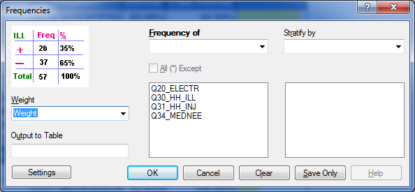
Once weights are assigned, frequencies can be calculated for each of the interview questions. To calculate frequencies in Epi Info™ 7 “classic mode”, read (import) the data file with the weight that was just created. Click on “Frequencies” along the left hand column. In the “frequency of” box, select each variable for which you would like results and, in the “weight” box, select the variable “WEIGHT” that was just created. Finally, click “OK” (Figure 12) and a report will be generated providing the estimates.
Figure 12. Epi Info™ 7 “classic mode” frequency analysis window showing selected variables and weight.

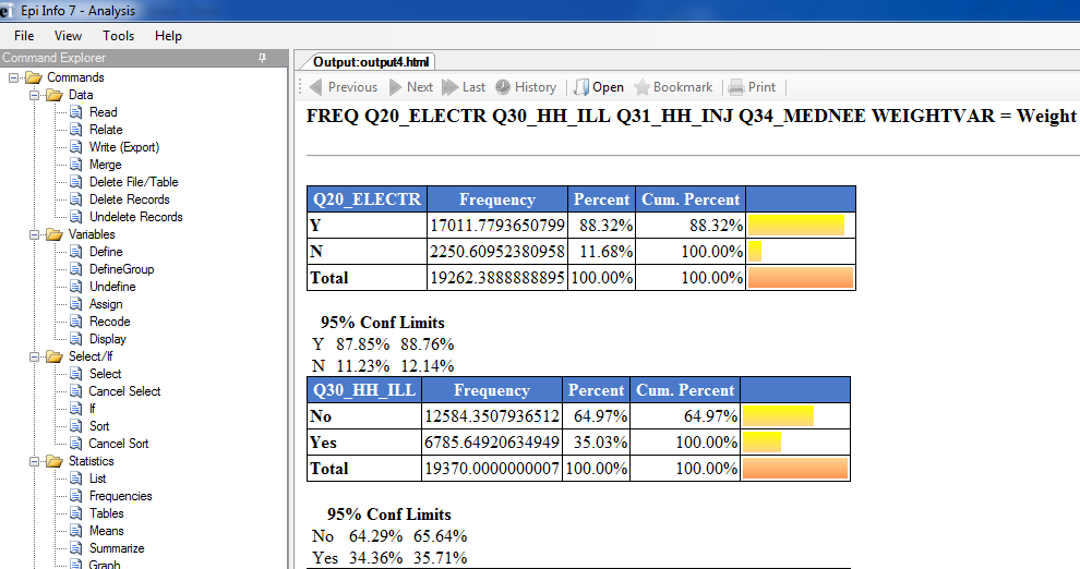
Figure 13 displays the Epi Info™ output window with the selected variables, followed by a table for each selection. These output tables should be saved for use in the report.
Figure 13. Example of Epi Info™ 7 “classic mode” output window showing weighted frequencies

To obtain unweighted estimates, follow the above instructions, but do not assign a variable in the “weight” box. Applying the weights provides projected estimates that can be generalized to every housing unit in the assessment area or sampling frame. Table 7 shows the unweighted and weighted frequencies for a specific question from the 2009 Kentucky Ice Storm CASPER.
Table 7. Unweighted and weighted frequencies of current source of electricity following the Ice Storms, Kentucky, 2009
|
Weighted |
|
|
|
|
|
||
|
Unweighted |
|
Weighted |
|||||
Characteristic |
Frequency |
Percent |
|
Frequency |
Percent |
95% CI |
||
Source of Electricity |
|
|
|
|
|
|
||
Power company |
137 |
74.1 |
|
14190 |
74.0 |
61.9-86.0 |
||
Gasoline generator |
29 |
15.7 |
|
3200 |
16.7 |
7.6-25.7 |
||
None |
19 |
10.3 |
|
1789 |
9.3 |
3.8-14.8 |
||
Remember that weighted analysis does not account for the changes that may occur in the number of households between the time of the census and the time of the assessment (e.g., the number of households per cluster may have changed between 2000, when the census was conducted, and 2009, when the CASPER was conducted). Therefore, despite attempts to present unbiased estimates, the frequencies reported might lack precision.
5.3 Calculation of 95% confidence intervals
The 95% confidence intervals (CIs) should be provided with the weighted estimates. These confidence intervals indicate the reliability of the weighted estimate. Follow these steps to calculate 95% confidence intervals in Epi Info™ 7:
Open Epi Info 7 in classic mode (Figure 14).
Figure 14. Classic mode of Epi Info 7
Read (import) the data file.
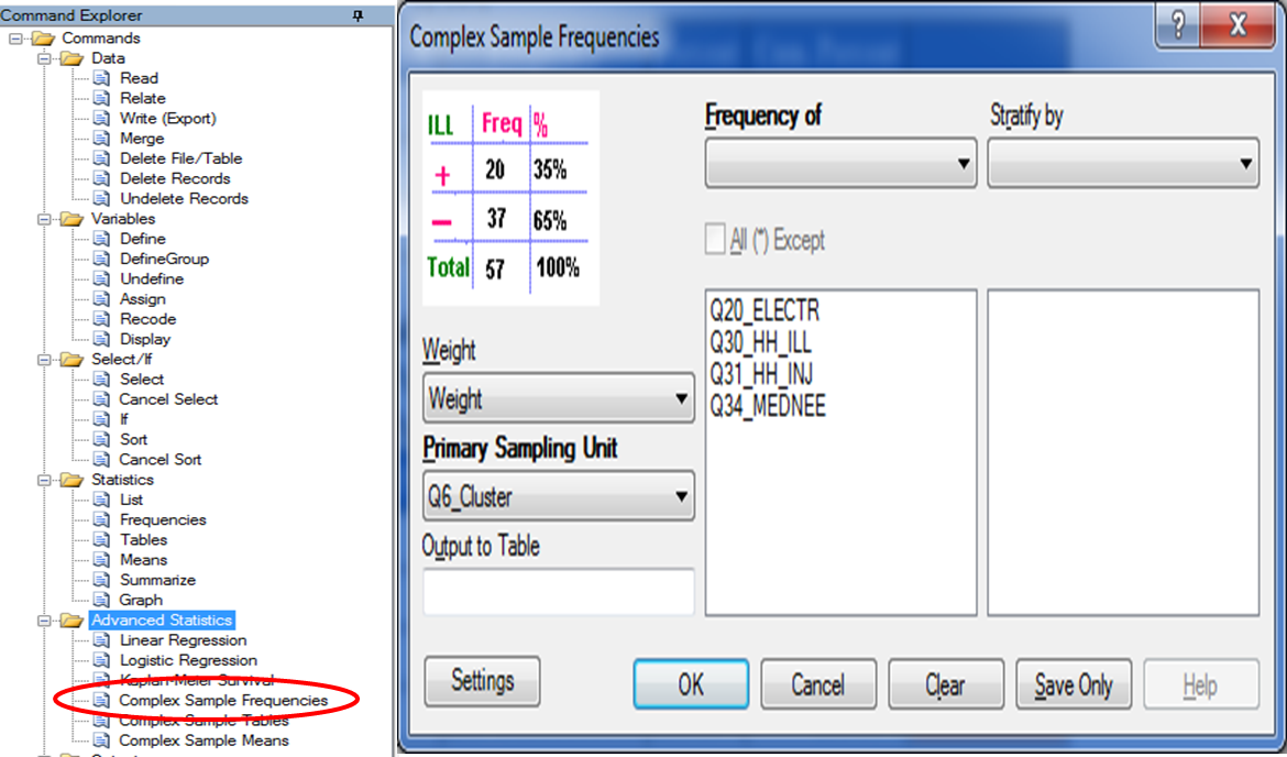
Select “Complex Sample Frequencies Command” under advanced statistics, and in the dialog box for Frequency, select the variable(s) in which you are interested (Figure 15).
Figure 15. Selected variables for calculation of complex sample frequencies (sample data)

Under the Weight drop-down menu, select the “weight” variable for calculating the weighted CI.
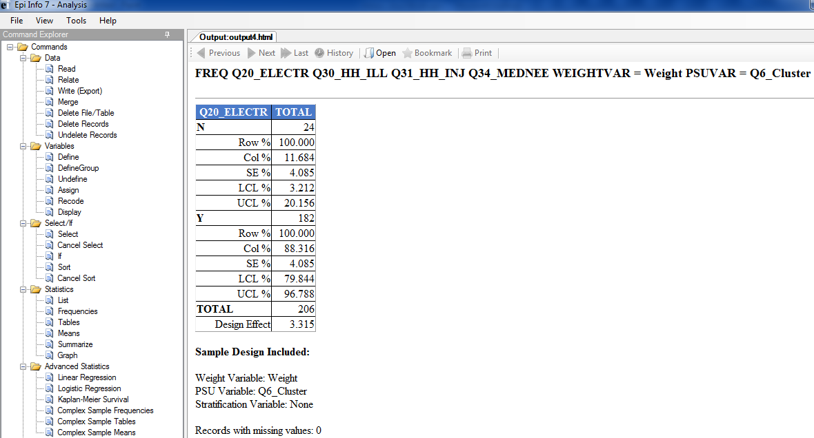
Under PSU, select the “Cluster Number” variable and Click OK (Figure 16).
Figure 16. Example of 95% CI output in Epi Info™ 7 “classic mode”

Right-click on the table and select “Export to Microsoft Excel”.
| File Type | application/vnd.openxmlformats-officedocument.wordprocessingml.document |
| Author | Nicole Nakata |
| File Modified | 0000-00-00 |
| File Created | 2021-01-23 |
© 2026 OMB.report | Privacy Policy
