CMS-10178.Supporting Statement Part B
CMS-10178.Supporting Statement Part B.doc
Payment Error Rate Measurement in Medicaid & Children's Health Insurance Program (CHIP)
OMB: 0938-0994
Supporting Statement – Part B
Collections of Information Employing Statistical Methods
1. To measure improper payments for PERM, 17 States from a total of 50 States plus the District of Columbia (i.e., ‘51’ States) were selected each year to create a three year rotation cycle. The States were rank-ordered by their past Federal fee-for-service (FFS) expenditures and grouped into the four strata of 17 States each for three PERM cycles (3x17=51). This distribution of States is shown in Table 1.
Table 1: State Strata Defined
-
Stratum
Cycle 1
(FY 09,12,15)
Cycle 2
(FY 10,13,16)
Cycle 3
(FY 11,14,17)
1A
3
3
3
1B
3
3
2
2
6
5
6
3
5
6
6
Total
17
17
17
For the FY 2012 (Cycle 1) and later PERM cycles, a service-type stratification approach is used for the FFS sample. Strata within each State FFS universe will consist of service-type strata. These strata will have equal sample sizes, but the total dollars in each stratum will differ, depending on the total dollars associated with that service type in the claims universe.
Step 1: All payments in the FFS universe are assigned to one of the service categories:
Step 2: Within each stratum, all lines are sorted from largest to smallest payment amounts
Step 3: An equal number of lines is sampled from each of the strata.
The managed care universe will continue to be stratified by paid amount, as it was in prior cycles
On February 4, 2009, the Children’s Health Insurance Program Reauthorization Act of 2009 (CHIPRA) (Pub. L. 111-3) was enacted. Section 601(f) of the CHIPRA requires CMS to establish State-specific sample sizes for application of the PERM requirements with respect to CHIP for fiscal years beginning with the first fiscal year that begins after the date on which the new final rule is in effect for all States, on the basis of such information as the Secretary determines appropriate. In establishing such sample sizes, the Secretary shall, to the greatest extent practicable: (1) minimize the administrative cost burden on States under Medicaid and CHIP; and (2) maintain State flexibility to manage such programs. CMS published the final PERM rule on August 11, 2010 (75 FR 48815), therefore the State-specific sample size for PERM, although the execution of these responsibilities remains with CMS and the Federal contractors, not the States. Under the Secretary’s authority at section 1102(a) of the Act and in order to effectively implement the IPERA, CMS applied these sampling procedures to both Medicaid and CHIP.
In addition, CMS also established a maximum sample size of 1,000 claims for each component. Because reviewing claims requires both staff and monetary resources, a maximum sample size puts a limit on expenditures. Statistical tests suggest that if State-level precision cannot be met with a sample size of 1,000 claims, it is unlikely to be met with any reasonable sample size; however, a substantial increase in the probability of reaching precision goals can be gained by increasing the sample size for 500 to 1,000.
The Statistical Contractor will estimate State-specific sample sizes for each program component within each State based on the prior cycle’s error rate (with the exception of FY 2007 and FY 2008 CHIP programs that elected not to accept a component of their CHIP PERM error rates from those cycles; if a State does not accept the component rate from the FY 2007 or FY 2008 cycle, the next measurement cycle for that State will be considered the “base year” for purposes of determining the State-specific sample size). The State specific sample size must be sufficient to meet the precision requirements, which is to estimate the component error rate with a 95 percent confidence interval f 3 percentage point in either direction.
The base sample sizes are 520 for Medicaid FFS and CHIP FFS (base of 500 and 20 additional oversample) and 240 for Medicaid Managed Care and CHIP Managed Care ( base 240 and 20 for additional oversample),
All sampled FFS claims receive a data processing review; sampled FFS claims that are not denied or Medicare crossover claims receive medical review. Sampled managed care claims receive only a data processing review. The final FY 2008 and FY 2009 PERM payment error rate reports will contain national Medicaid and CHIP rates that include FFS, managed care, and eligibility components, as prescribed by Public Law 107-300
The anticipated response rate for all facets of PERM should approach 100% due to the regulatory requirement under Final Rule CMS 6062-F 42 CFR 431.970. Previous periods of performance of PERM have shown that most States comply at the 100% level for their programs.
2. The overarching procedures for the collection of information, including sample selection and stratification, are described in #1 above. 1 FFS samples were determined to need to contain approximately 1,000 claims per State program, using an assumed error rate of up to a maximum of approximately 10% and ten strata used for sampling. The maximum error rate parameter was based on the FY 2006 PERM results, the early FY 2007 results, and the tendency for error rates to decrease over time due to the responsible agencies learning the operationalized program. Under these conditions, the federal precision requirements should be met, which include no more than an anticipated +/- 3% margin of error at a 95% confidence level for payment error rates at the State program level, and no more than an anticipated +/- 2.5% margin of error at a 90% confidence level for payment error rates at the national program level.
In more statistical depth, sample size determinations follow the approach outlined in Cochran (1977). The process starts with a variance estimation. The total variance for a staged sampling model from Cochran is as follows (of note, Cochran shows a two-stage model, whereas the variance for a three-stage sample nests Cochran’s equation within one more stage to account for payment method, FFS or managed care): 2, 3
(1)![]()
where:
N=total States in universe
n=total States sampled
f1=proportion of States sampled
Yi=projected dollars in error for a State
Mi=total units in State i
mi=total units sampled in State i
f2i=proportion of units sampled from State i
S2i2=sample variance of errors within State i
The goal is to determine the expected value of the variance of the projected dollars in error.
Letting
(2) σYB2 =![]()
denote the variance in projected error between States, using the identity Yi=RiPi, and assuming that all Ri are equal, then σYB2=R2* σPB2, where σPB2 is the variance in payments between States.
(3) Next, for each State-level estimate, the variance of the error rate is given by:
(4)
where Pi is the total payments for the State, and σEW2 is the variance of the projected dollars in error within a State.
The goal is to determine the expected variation in projected dollars in error within a State, which depends on the State selected (the first stage).
Therefore:
(5)![]()
which is attained only when assuming independence between the error rate and payments, and this appears to be a reasonable assumption.
Additionally, note that σRi2 is currently designed such that the precision met is .03, with 95 percent confidence.4 For generality, the desired State level precision denoted as d, then note that σRi2=d2/z2 where z is the standard normal of a designated level of confidence.
Combining this, equation (1) can be rewritten as:
(6)
![]()
All that remains is to find the variance of the error rate, which for the method used by the Office of Inspector General (OIG) (a “difference” estimator) would simply be:
(7)![]()
Note: The sample size calculations in these derivations were for simple random sampling schemes. For stratified random sampling schemes, the same procedure is used, partitioned into the respective strata, and each individual result combined in a standard fashion.
The overall formula for the sample size needed to construct a rate with a specified precision is given by:
![]()
where
zα/2 = the standard normal value with α/2 in one tail of the distribution.
d = desired precision
k = coefficient of variation, assumed constant across strata
π = probability a sampled unit is in error, assumed constant across strata
The formula above provides the overall sample size requirement for the study, and this sample size would be divided into strata. These particular calculations assume that the sample will be allocated based on the proportion of payments in each stratum. Note: The value of π is technically the probability that a sampled unit (e.g., line item) is in error, and is not the dollar weighted error rate. In practice; however, the statistical contractor would use the dollar valued error rate in lieu of this value.
Sampling with strata is done as follows:
Sorted the data first by paid amount
Calculated the total payments for universe
Defined strata: sorted claims in descending order, such that each stratum represents 10 percent of expenditures
Determined the skip factor for each stratum (denoted by ki).
Let
![]() denoted the universe number of claims for the ith stratum
in a State
denoted the universe number of claims for the ith stratum
in a State
![]()
Determined a random start value for each stratum (denoted by starti), such that
 (i denotes the ith strata)
Sampled every
 th
item within the ith stratum
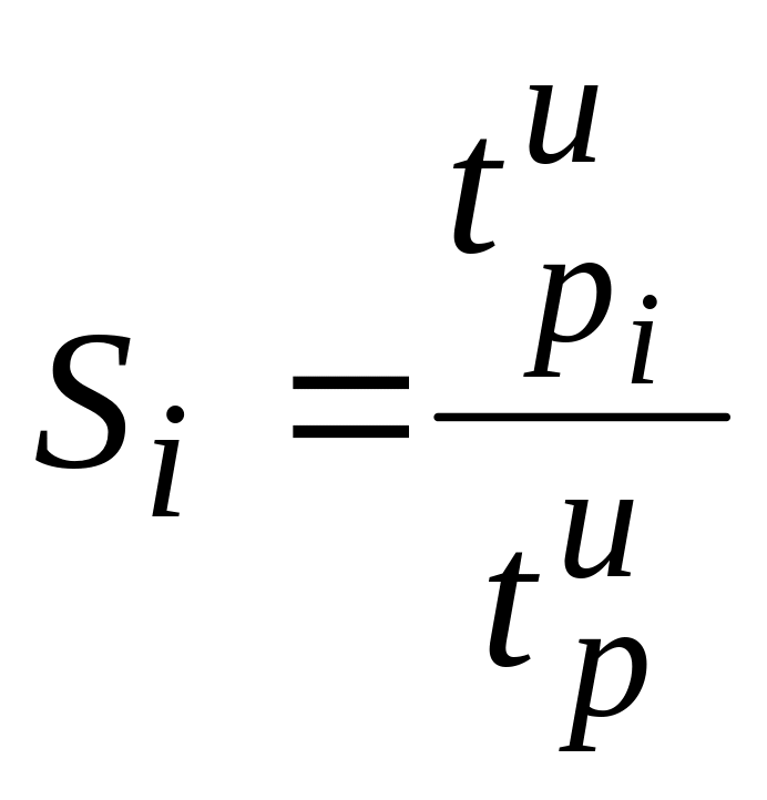
The estimation procedure thus accounts for the nesting of claims within payment methods within program types within States. The error rate calculations utilize the Intra-class Correlation Coefficient to properly adjust for similarities within the nested structures in the data. In doing so, the PERM SC has chosen to use a Separate, Separate, Combined Estimator (SSC). This method represents a mixture of two methods: the combined ratio estimator and the separate ratio estimator. It is not documented in standard sampling textbooks, but the estimator and its standard error are straightforward to formulate and have been used for PERM in FY 2006 and FY 2007. The discussion is divided into the three steps for the estimator.
Stage 1: SRE for Combining Stratified Results
First, the PERM sample design has four State strata, determined by their expenditure amounts. The estimates and standard errors can be assumed to be produced for each State stratum.
The SR estimator is given by:
(10)![]()
where
 share
of expenditures for State stratum i (sum across all strata equals 1)
![]() error rate for stratum i, as determined by a ratio estimator, to be
described later
error rate for stratum i, as determined by a ratio estimator, to be
described later
i denotes the State stratum (i=1 to 4)
The variance for the SSC is given by:
(11)![]()
Note the variance of the stratum specific error rate will be derived in later steps.
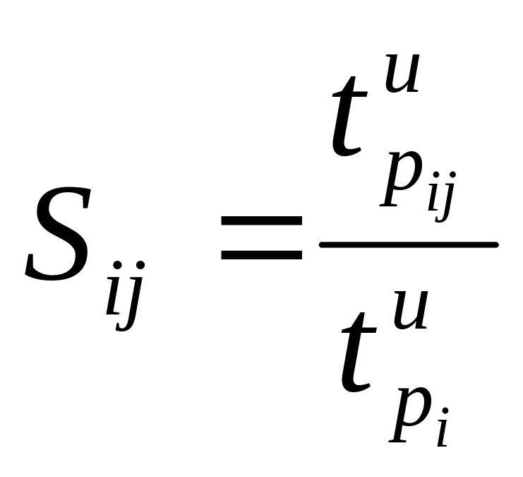
Stage 2: SR estimator for State Stratums
Within each State stratum, individual rates are estimated. The application of the separate ratio estimator occurs again when creating these State stratum rates. The State stratum rate will be the weighted combination of the State specific rates, with the weights being the relative shares of expenditures. Therefore,
(12)![]()
where
 share
of expenditures for State j in State stratum i (sum of all strata
equals 1)
![]() error rate for State j in stratum i, as determined by a ratio
estimator, to be described later
error rate for State j in stratum i, as determined by a ratio
estimator, to be described later
i denotes the State stratum (i=1 to 4)
j denotes the State (i=1 to ni)
The variance follows the properties of a three stage sample design, where the selection of States is the first stage, the selection of program type is the second stage, and the selection of the sampling units (claims) within payment method is the third stage. The variance of this portion of the estimator is given by:
(13)![]()
Let
(14)![]()
such that
(15)![]()
Then continuing from (13),
(16)
![]()
The estimated variance is given by
(17)
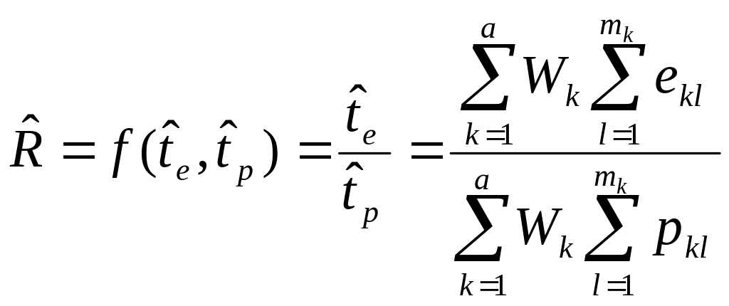
Stage 3: Combined estimator for State Stratums
Where
![]() can
vary based on the estimator employed for estimating rates at the
State level. For the combined ratio estimator, the State level error
rates are estimated by:
can
vary based on the estimator employed for estimating rates at the
State level. For the combined ratio estimator, the State level error
rates are estimated by:
(18)
where:
![]()
![]()
mk are the number of claims sampled from strata k
Mk are the number of claims or line items in the universe from strata k
ekl represents the error on the lth claim in the kth stratum
pkl represents the payment on the lth claim in the kth stratum
Then estimated variance is given by:
(19)

The needed accuracy is provided by the IPIA and should be no more than an anticipated +/- 3% margin of error at a 95% confidence level for payment error rates at the State program level, and no more than an anticipated +/- 2.5% margin of error at a 90% confidence level for payment error rates at the national program level.
On occasion, the distribution of claims within a universe can lead to the dollar value of a single or a small number of claims comprising over 10% of the State’s universe of claims. Under that condition, the 10-strata structure is maintained and the claims that would have been sampled from the stratum, if it had contained enough claims, are evenly spread across the remaining strata.
On other occasions, States are late with some data for varied reasons. The PERM SC has implemented a roll-over policy to sample the claims along with those from later submissions, rather than to create a supplemental sample. The reason is that the statistical properties of the rolled-over sampling units are more closely aligned with the theoretically optimal properties than they are under the condition of a supplemental sample.
In order to meet the requirements of IPIA, all selected States must fully participate.
3. Most States have been quite responsive, so non-response is a minimal issue for PERM. The accuracy and the reliability for PERM are specified by federal regulations and supported by appropriate sample sizes. For these reasons, the information collected should be appropriate for its intended purposes. Reliable data are expected because the PERM SC compares the States’ data with their CMS 64 and CMS 21 submissions for Medicaid and CHIP, respectively. Further, States are subject to an OMB audit on their PERM submissions.
4. Not applicable.
5. Contact information
The Lewin Group
3130 Fairview Park Drive
Falls Church, VA
Fax: (703) 269-5705
1 A stratified sample is simply a series of simple random samples, combined together.
2 Note: In practice, PERM will utilize a slightly different estimator that utilizes the error rate for each State, as opposed to the projected dollars in error for each State. However, the above formula could be used as well, and the resulting sample size calculation of States would yield similar results with a much simpler presentation herein.
3 The number on the equations is the original found in Cochran (1977).
4 In the FY 2007 error rate, the precision at the State level will be less than this because of reductions in sample sizes.
| File Type | application/msword |
| File Title | Supporting Statement – Part B |
| Author | CMS |
| Last Modified By | WILLIAM PARHAM |
| File Modified | 2016-09-28 |
| File Created | 2016-09-28 |
© 2026 OMB.report | Privacy Policy