Attachment V - Assessing Nonresponse Bias in the Consumer Expenditure Interview Survey

The Consumer Expenditure (CE) Survey is a nationwide household survey conducted by the U.S. Bureau of Labor Statistics to find out how U.S. consumers spend their money. The CE Survey actually consists of two sub-surveys, a quarterly Interview survey, and a two-week Diary survey. The Interview survey provides detailed information on large expenditures such as property, automobiles, and major appliances, as well as on recurring expenditures such as rent, utilities, and insurance premiums. By contrast, the Diary survey provides detailed information on the expenditures of small, frequently purchased items such as food and apparel. The data from the two surveys are then combined to provide a complete picture of consumer expenditures in the United States.

Over the past ten years (2007-2016) the response rates for the Interview and Diary surveys decreased by more than ten percentage points, from 74 percent to 63 percent in the Interview survey, and from 73 percent to 57 percent in the Diary survey. These decreases are a concern because respondents and nonrespondents may have different kinds of expenditures, and if that is true then there may be a bias in favor of the respondents’ expenditure patterns with the decreasing response rates increasing the amount of bias.

The Office of Management and Budget (OMB) encourages all federal surveys to study their nonresponse bias, and OMB requires such a study of all federal surveys whose response rates are below 80 percent.¹ Both the CE Interview and Diary surveys have response rates below 80 percent, so a nonresponse bias study is required of them.² OMB’s directive (2006) requires an analysis of nonresponse to determine whether the data are “missing completely at random” (MCAR), and another analysis to estimate the amount of nonresponse bias in the survey’s estimates.³ Both analyses are summarized in this report.

The research presented in this report updates and expands research that was performed ten years ago by CE program staff in which it was found that the expenditure estimates from the Interview survey did not have a significant amount of nonresponse bias even though the respondents and nonrespondents had different characteristics, and even though the data were not MCAR.^⁴

This report contains a summary of four studies undertaken with more recent data to respond to OMB’s directive about determining whether CE’s data are MCAR. The four studies are:

Study 1: a comparison of CE’s respondent demographic characteristics to those of the American Community Survey (ACS);
Study 2: a comparison of response rates between subgroups of CE’s sample;
Study 3: a linear regression analysis of CE’s response rate trends and demographic characteristic trends over the ten-year period 2007-2016;
Study 4: a logistic regression analysis of CE’s response rates using socio-demographic variables that are available for both respondents and nonrespondents.

All four studies address the MCAR issue and conclude that the data in both surveys are not MCAR. Study 1 and Study 3 show the distributions of various socio-demographic characteristics differ between the CE and ACS surveys, and that the relationships between some of them are changing over time. Study 2 and Study 3 show the response rates among various subgroups in the CE’s sample differ from each other and the relationships between some of them are changing over time as well. And Study 4 shows that CE’s overall response rate is affected by the demographic composition of the survey’s sample. All four of these studies show that different subgroups of the survey’s sample respond to the CE surveys at different rates, which means their patterns of “missing-ness” are different, and therefore the surveys’ nonresponders and their data are not MCAR.

Specific findings include lower-income respondents being over-represented and higher-income respondents being under-represented in both CE surveys; rural areas having higher response rates than urban areas in both CE surveys; and homeowners having lower response rates than renters in the Interview survey but higher response rates in the Diary survey. Finally, the linear regression analysis shows that some of these relationships are changing over time. These findings reinforce the conclusion that the data in both CE surveys are not MCAR.

In addition, this report analyzes the results of four methods undertaken with more recent data to respond to OMB’s updated 2016 guidelines about determining the amount of nonresponse bias in the CE Interview and Diary Surveys. OMB’s guidelines for nonresponse bias require comparisons between respondents and nonrespondents but since no expenditure data is available for CE’s nonrespondents, several approaches have been developed to quantify the bias. The calculation of the statistic for nonresponse bias is derived from the formula, for each of four methods used for estimation. is the nonresponse bias of the respondent sample mean, is the base-weighted mean calculated from all sample respondents, and is the adjusted mean calculated from all sample respondents but using data from all sample cases. Methods 1, 2, and 3 assume that nonresponse is Missing At Random (MAR)^⁵ while Method 4 does not.

The four methods are as follows:

Method 1: This method estimates nonresponse bias by comparing expenditure estimates from the survey’s respondents when they are weighted two different ways – with unadjusted base weights and with base weights adjusted to account for nonresponse. The nonresponse adjustment is the one used in CE’s published expenditure estimates.
Method 2: This is identical to Method 1 except the base weights are adjusted in a different way. They are adjusted with a logistic model of nonresponse instead of CE’s official method of adjustment for nonresponse.
Method 3: This method is identical to Method 2 except the logistic model has an additional variable.
Method 4: This method estimates nonresponse bias by comparing expenditure estimates from two different subsets of CE’s respondents, “proxy respondents” and “proxy nonrespondents.” Some households respond to the CE survey more readily than others, and “proxy respondents” are those that respond more readily, while “proxy nonrespondents” are those that respond less readily, as measured by the number of contact attempts.

Each of the four methods have strengths and weaknesses so picking one over the other is subjective. The report will describe each method and provide tables and graphs that highlight the magnitude of the bias and trends over the ten-year period.

The report summarizes the relative bias for the major expenditure summary variables for both the Interview and Diary surveys and covers the same ten-year period. There is agreement in the Interview survey among Methods 1, 2, and 3, which shows statistically significant presence of negative relative bias^⁶ of -0.5 percent to -1.5 percent for the total expenditures summary variable, ZTOTALX4. Several of the other major summary variables for the Interview survey show similar patterns for these same three methods. However, applying these methods to the Diary Survey shows a statistically significant presence of positive relative bias in the range of 0.5 percent to 2 percent. This is especially apparent for Method 2 and Method 3 for the Diary survey total expenditure summary variable, ZTOTAL. Furthermore, Method 2 shows a strong presence of positive relative bias for all of the Diary survey summary variables while the other three methods show varying levels of positive relative bias over the ten-year period. Research for this report was conducted under the concept that the data were MAR.

1. Introduction and Approach

As mentioned earlier, over the past ten years the response rate for the Interview survey decreased from 74 percent to 63 percent, and the response rate for the Diary survey decreased from 73 percent to 57 percent. This decrease is a concern because it may affect the accuracy of CE’s expenditure estimates. Table 1 below shows the response rate history for both surveys over the past ten years.

Table 1. Unweighted Response Rates for the CE Interview and Diary surveys, 2007-2016


	CE Interview Survey				CE Diary Survey

Collection Year	Total Eligible Cases	Type A Noninterviews	Complete Interviews	Response Rate	Total Eligible Cases	Type A Noninterviews	Complete Interviews	Response Rate
2007	37,016	9,681	27,335	73.8%	19,595	5,848	13,747	70.2%
2008	37,302	9,757	27,545	73.8%	19,710	5,531	14,179	71.9%
2009	37,623	9,594	28,029	74.5%	20,024	5,400	14,624	73.0%
2010	38,718	10,289	28,429	73.4%	19,988	5,692	14,296	71.5%
2011	38,348	11,358	26,990	70.4%	19,823	5,898	13,925	70.2%
2012	38,835	11,842	26,993	69.5%	20,298	6,537	13,761	67.8%
2013	39,142	13,034	26,108	66.7%	20,296	7,961	12,335	60.8%
2014	39,003	13,095	25,908	66.4%	20,476	7,170	13,306	65.0%
2015	36,692	13,118	23,574	64.2%	20,517	8,676	11,841	57.7%
2016	40,375	14,934	25,441	63.0%	20,391	8,839	11,552	56.7%

To determine whether the missing values in the two CE surveys are MCAR, four studies mentioned in the Executive Summary were performed and elaborated below. But before going any further, the term “missing completely at random” needs to be defined. The generally accepted definition comes from Roderick Little and Donald Rubin. According to them, data are “missing completely at random” (MCAR) if the mechanism that produces the missing values is unrelated to the values of the data themselves. More precisely, data are “missing completely at random” if their pattern of “missing-ness” is independent of the data’s actual values and the values of any other variables (Little and Rubin, 2002).⁷ The question of whether the data are MCAR is important because nonresponse bias is often associated with the data not being MCAR.

In practical terms, this definition means CE’s data are MCAR if the survey’s respondents and nonrespondents spend the same amount of money on the same set of goods and services (i.e., the pattern of “missing-ness” is independent of the data’s actual values), and if every demographic subgroup of the survey’s sample has the same response rate (i.e., the pattern of “missing-ness” is independent of any other variables). In general, the amount of money nonrespondents spend on various goods and services is unknown since nonrespondents do not respond to the survey, so the main question is whether every demographic subgroup has the same response rate. If so, then the missing data might be MCAR, depending on the expenditures of the respondents and nonrespondents, but if they have different response rates then the missing data are not MCAR because the mechanism that produces the missing values is not independent of the demographic subgroups. Examining the response rates of different demographic subgroups is one of the primary methods of determining whether a survey’s data are MCAR, and it is used in this report.⁸

The first study to determine whether the data are MCAR compares the distribution of socio-demographic characteristics of the survey’s respondents to those of a recent census or a “gold standard” survey. The ACS can be thought of as a gold standard survey.⁹ Any differences between the survey and the gold standard survey suggest that they have different response mechanisms, and since the “gold standard” survey is presumed to have a response mechanism closer to that of an MCAR process, the other survey is presumed to have a response mechanism further from that of an MCAR process, which means its data’s “missing-ness” pattern is probably not independent of the data themselves.

The second study to determine whether the data are MCAR compares the survey’s respondents and nonrespondents to each other according to a few socio-demographic variables that are available for both groups. Any differences between them indicate that the pattern of “missing-ness” is not independent of other variables, and therefore the missing data are not MCAR. In spite of the limited number of variables that can be used in this analysis, it is another standard method of determining whether the data are MCAR, and it is used in this report.

The third study looks at ten-year trends in response rate and demographic characteristic “relativities” using simple linear regressions to determine whether the relationships of the response rates to each other and the demographic characteristics to the ACS (the gold standard survey) are changing over time. In the case of response rates, the relativities are computed as the response rate for a subgroup of CE’s total sample divided by the response rate for the total sample itself. For example, the response rate relativity for the Northeast region of the country would be the response rate for the Northeast region divided by the response rate for the whole country. In the case of demographic characteristics, they are computed as the percentage of CE’s respondents in a certain demographic subgroup divided by the ACS’s estimate of the percentage of the population in the same demographic subgroup.

Finally, the fourth study uses logistic regressions to determine whether the surveys’ response rates are affected by certain socio-demographic variables. A logistic regression is a model of the outcomes of a binary process, such as whether a sample household participates in the CE survey. It has a specific algebraic form that ensures its numeric values are between 0 and 1, which makes it suitable for modeling probabilities:

Simple algebra allows the model to be rewritten like this:

which shows how it can be written as an ordinary linear regression. That allows the methods of ordinary linear regressions to be used to estimate the model’s parameters and other statistical properties of the model.

All four of these studies show that CE’s data are not MCAR.

2. Methodology

2.1. Data

For comparability of results, the analyses for the Interview and Diary surveys used the same ten years of data, which was January 2007 through December 2016. The unit of analysis in these studies was generally the consumer unit (CU), but a mixture of CU and person level respondents (individual CU members) was used for the analysis comparing CE’s demographic characteristics to those of the ACS. CUs are basically the same thing as households.¹⁰

2.2. Weighting

The CE survey’s sample design is a nationwide probability sample of addresses. That means a random sample of addresses is selected to represent the addresses of all CUs in the nation. As mentioned earlier, most addresses have only one CU living there, hence the terms “address” and “CU” are often used interchangeably. Each interviewed CU represents itself as well as a number of other CUs that were not interviewed for the survey and therefore each interviewed CU must be weighted to properly account for all CUs in the population.

In CE’s sample design, a random sample of geographic areas called Primary Sampling Units (PSUs) is selected for the survey, and then a random sample of CUs is selected from those PSUs to be in the survey. The Bureau of Labor Statistics (BLS) selects the sample of PSUs, and then the U.S. Census Bureau selects the sample of CUs and provides their base weights, which are the inverse of the CU’s probability of selection. Each CU in a PSU has the same base weight. Then BLS makes three types of adjustments to the base weights: an adjustment in the rare situation where a field representative finds multiple housing units where only a single housing unit was expected; a noninterview adjustment to account for CUs that were selected for the survey but did not participate in it; and a calibration adjustment to account for nonresidential and other out-of-scope addresses in the sampling frame as well as sampling frame under-coverage.¹¹ These weight adjustments are made to each individual CU that participated in the survey. All of the studies in this report use base weights, but the study comparing CE respondents to external data use all three weights (base weights, noninterview adjustment weights, and final calibration weights).

2.3. Significance tests for one-way and two-way socio-demographic comparisons

Respondents and nonrespondents were compared on several categorical socio-demographic characteristics to determine whether the two groups had the same distribution of characteristics, and whether those characteristics were correlated with their likelihood of responding to the survey. For these comparisons, the Rao-Scott chi-square statistic was used, which is a design-adjusted version of the Pearson chi-square statistic involving differences between observed and expected frequencies. For one-way comparisons, the null hypothesis was that the respondents in the CE and ACS surveys had the same distribution of characteristics. And for two-way comparisons, the null hypothesis was that the response status (interview or noninterview) of CUs in the CE survey was independent of their socio-demographic characteristics.

Ten years of data were analyzed in this study (2007-2016), with a separate analysis done for each year. That means ten Rao-Scott chi-square statistics were generated for each comparison, with one statistic generated for each year, and the results of those ten yearly analyses were summarized by counting the number of times statistically significant results were obtained. For one-way comparisons, a comparison was considered to be “strongly significant” if 5 or more years had statistically significant differences (p<0.05); “moderately significant” if 3-4 years had statistically significant differences; and “not significant” if 0-2 years had statistically significant differences. For example, the difference between CE’s and ACS’s household “tenure” (homeowners versus renters) distributions were statistically significant in 6 of the 10 years for the Interview survey and in 7 of the 10 years for the Diary survey, so both comparisons were considered to be “strongly significant” (see Appendix B).

For two-way comparisons, the scoring system was similar to the one-way comparisons. For each comparison, a net difference was calculated as the number of years the first subgroup listed had a statistically significantly higher response rate than the second subgroup listed (p<0.05) minus the number of years it had a statistically significantly lower response rate (p<0.05). In other words, for each year, if the first subgroup listed had a statistically significantly higher response rate than the second subgroup listed, then it was given a score of “+1”; if it had a statistically significantly lower response rate, then it was given a score of “–1”; and if there was no statistically significant difference, then it was given a score of “0.” Then the ten scores for the ten years were summed, giving an overall score between –10 and +10. The difference between the two subgroups was then categorized as “strongly significant” if the overall score was greater than or equal to +5 or less than or equal to –5; “moderately significant” if it was equal to +3, +4, –3, or –4; and “not significant” if it was between –2 and +2. Here is an example comparing the response rates for the South region to the West region of the country:

Category	# Years	Score
South’s response rate is significantly higher than the West’s response rate	7 years	7(+1) = +7
South’s response rate is significantly lower than the West’s response rate	1 years	1(–1) = –1
No significant difference between the South’s and West’s response rates	2 years	2( 0) = 0
Overall Score		+6

The overall score was +6, which was greater than or equal to +5, hence the South’s response rates were higher than the West’s response rates, and the difference was “strongly significant.”

2.4. Significance tests for linear regression analysis

For tests of significance pertaining to response rate subgroups, “relativities” were calculated as the ratio of each demographic subgroup’s response rate to the overall response rate, with one such ratio calculated for each of the ten years. Then a linear regression line Y = β₀ + β₁X was fit to the data where the x-variable was the year in which the data was collected, and the y-variable was the response rate relativity for that year. After fitting the line, a t-test was performed to determine whether its slope differed from zero. The two-sided hypothesis test of the slope was this:

H₀: β₁ = 0

H_a: β₁ ≠ 0

As mentioned earlier, a level of significance of α=0.05 was used, so if the t-test yielded a p<0.05 the slope of the regression line was considered to be significantly different than 0. If the slope was positive it was considered a statistically significant positive slope and if the slope was negative it was considered to be a statistically significant negative slope.

3. Individual studies to determine MCAR

3.1. Comparison of respondents to external data

As mentioned earlier, a common approach to analyzing the effect of nonresponse on a survey’s estimates is to compare the distribution of socio-demographic characteristics of the survey’s respondents to that of a recent census or other “gold standard” survey (Groves, 2006).

Appendix A for the Interview survey and Appendix D for the Diary survey show a 2016 comparison of the distribution of selected socio-demographic characteristics between the CE and ACS surveys. The characteristics compared are gender, age, race, education, CU size, housing tenure, number of rooms in a housing unit, owner-occupied housing value, monthly rent, and CU income. Housing information about the number of rooms in a housing unit, the housing unit’s market value, and the housing unit’s rental value are available from the Interview survey only. Tables for all years were produced but showing one year provides information to get a sense for the work that was done.

Comparing the distribution for a particular characteristic in the CE data to its distribution in the ACS data falls into the framework of a one-way Chi-square goodness-of-fit test. The Rao-Scott Chi-square statistic described earlier is used to determine whether a characteristic’s distribution in the CE and ACS surveys are the same or different. For both surveys, statistically significant differences (p < 0.05) were found for almost all of the socio-demographic characteristics regardless of whether the data was base-weighted, noninterview-weighted, or calibration-weighted. Table 2 below summarizes these results.

Table 2. A Comparison of Socio-Demographic Variable Distributions Between the CE and ACS Surveys
	CE Interview Survey versus ACS			CE Diary Survey versus ACS

	Base-weighted	Noninterview-weighted	Calibration-weighted	Base-weighted	Noninterview-weighted	Calibration-weighted
	Gender	Gender	Gender	Gender	Gender
	Age	Age		Age	Age
	Race	Race	Race	Race	Race	Race
“Strongly	Education	Education	Education	Education	Education	Education
Significant”	CU size	CU size	CU size	CU size	CU size	CU size
differences	Tenure	Tenure		Tenure
between	Income	Income	Income	Income	Income	Income
CE and ACS	Housing value	Housing value	Housing value
	Monthly rent	Monthly rent	Monthly rent
	# Rooms in housing unit	# Rooms in housing unit	# Rooms in housing unit
Moderately						Gender
Significant			Age
Not						Age
Significant			Tenure		Tenure	Tenure

It should be pointed out that there are factors beyond the characteristics of the respondents in these two surveys that make differences likely to be statistically significant. First, the large sample sizes of the CE Interview and Diary surveys as well as the ACS survey makes statistical significance likely even if the differences are relatively small. Second, the CE and ACS surveys differ in both their data collection modes and question wording. And third, for some of the CU-level variables examined, the definitional difference between CUs in the CE survey and households in the ACS may impact the results even though most of the time they are the same thing. As a result, the strength of the comparison of CE data with ACS data is limited by the extent to which the survey designs are truly comparable.

Further analysis was done to observe trends over time for the CE data compared to the ACS gold standard data by using a simple linear regression analysis on relativity measures over the ten-year period 2007 to 2016. The goal of this analysis is to determine whether the CE and ACS have the same distributions of socio-demographic characteristics, and if they are different whether they are getting closer to each other or moving apart from each other over time. In other words, whether the CE/ACS ratio is moving away from 1.00, moving towards 1.00, or staying the same distance from 1.00. The ten yearly relativities over the ten-year period 2007-2016 are plotted and analyzed to determine whether their relationships are changing or holding steady over time.

All of these analyses will be discussed in detail in the following four sections:

3.1.1. CE-to-ACS comparison for the Interview survey
3.1.2. CE-to-ACS comparison for the Diary survey
3.1.3. Regression analysis for the Interview survey
3.1.4. Regression analysis for the Diary survey

3.1.1. CE-to-ACS comparison for the Interview survey

As mentioned earlier, almost all of the characteristics have different distributions between the two surveys. Some of the differences are rather small and statistically significant only due to the surveys’ large sample sizes, but a few of them have noticeable patterns in which some socio-demographic subgroups are systematically over-represented or under-represented relative to the ACS survey. Characteristics with noticeable patterns include the market value of owner-occupied housing units, the monthly rent of rental housing units, and especially CU income that is shown below. The graphs below show the patterns of over-representation or under-representation for CU Income. The graphs show the socio-demographic subgroups along the horizontal axis, then above them there are ten circles showing the CE/ACS relativities for those subgroups for each of the ten years, and a solid line connecting the average value of the CE/ACS relativities to show the patterns.

CU Income. The first set of graphs shows the CUs’ annual incomes. The values range from $0 to $200,000+. The graphs show that CUs with low incomes are over-represented in the CE survey relative to the ACS survey, while CUs with high incomes are under-represented. CUs with incomes below $50,000 are over-represented by 5 to 20 percent, while CUs with incomes over $50,000 are under-represented by 5 to 20 percent. Furthermore, for CUs with high incomes, the under-representation grows with their incomes, so that, for example, the $100,000-$149,999 subgroup is under-represented in the CE survey, the $150,000-$199,999 subgroup is under-represented even more, and the $200,000+ subgroup is under-represented even more than that. Also, the graphs for the base-weighted data and the calibration-weighted data are nearly identical to each other, which shows that CE’s weighting procedures do not fix the problem.

CE-to-ACS Relativities for CU Income Subgroups in the Interview survey, 2007-2016

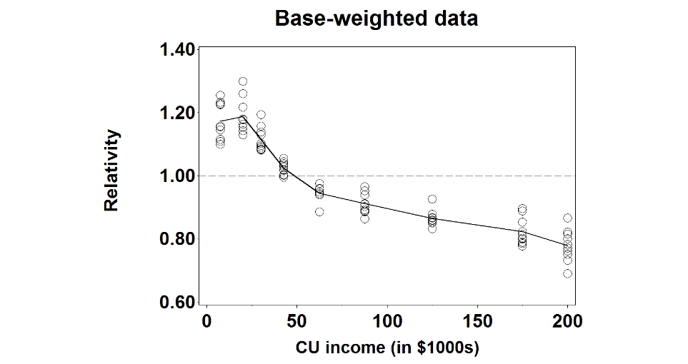
Summary. The three CE Interview survey socio-demographic categories involving money with CU incomes show similar patterns with the “wealthier” CUs being under-represented relative to the ACS survey, and the less wealthy CUs being over-represented. This is a problem since CE is a survey about money, and it may result in CE’s expenditure estimates being too low. Also, the graphs for the base-weighted data and the calibration-weighted data are nearly identical to each other, which shows that CE’s weighting procedures do not fix the problem (assuming there is a problem – that is, assuming ACS’s socio-demographic distributions are more accurate than CE’s socio-demographic distributions).

3.1.2. CE-to-ACS comparison for the Diary survey

Just like in the Interview survey, almost all of the characteristics have different distributions between the two surveys, although some of the differences are rather small and statistically significant only due to the surveys’ large sample sizes. However, a few of them have noticeable patterns in which some socio-demographic subgroups are systematically over-represented or under-represented relative to the ACS survey. Characteristics with noticeable patterns include CU income. The graphs below show the patterns of over-representation or under-representation for CU Income.

CU Income. The set of graphs below shows the CUs’ annual incomes. The values range from $0 to $200,000+. Just like in the Interview survey, the graphs show that CUs in the Diary survey with low incomes are over-represented relative to the ACS survey, while CUs with high incomes are under-represented. CUs with incomes below $50,000 are over-represented by 5 to 20 percent, while CUs with incomes over $50,000 are under-represented by 5 to 25 percent. Furthermore, for CUs with high incomes, the under-representation grows with their incomes, so that, for example, $100,000-$149,999 subgroup is under-represented in the CE survey, the $150,000-$199,999 subgroup is under-represented even more, and the $200,000+ subgroup is under-represented even more than that. Also, the graphs for the base-weighted data and the calibration-weighted data are nearly identical to each other, which shows that CE’s weighting procedures do not fix the problem.

CE-to-ACS Relativities for CU Income Subgroups in the Diary survey, 2007-2016

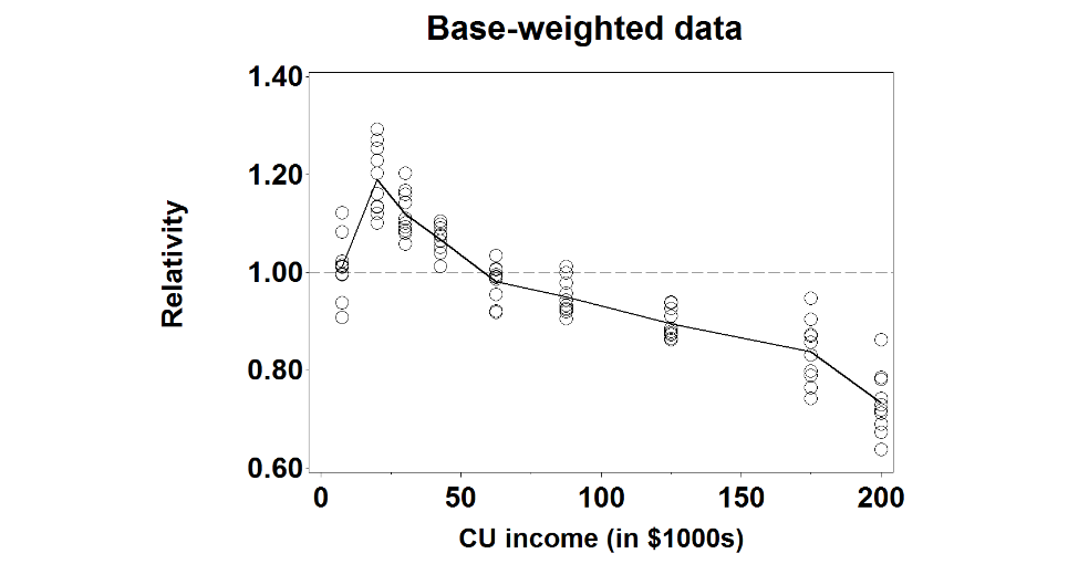
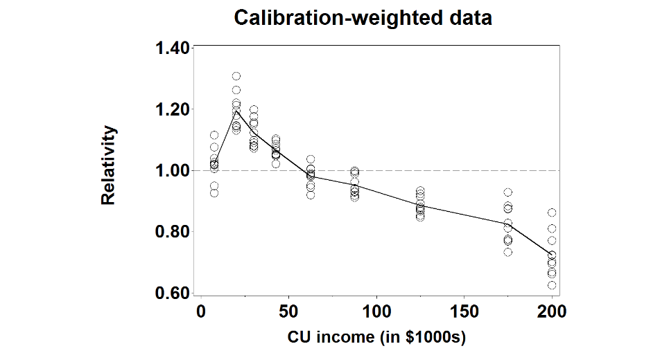
Summary. Just like in the Interview survey, CU income has noticeable patterns in which some of their subgroups are systematically over-represented or under-represented in the Diary survey relative to the ACS survey. The under-representation of CUs with high incomes is a problem since CE is a survey about money, and it may result in CE’s expenditure estimates being too low.

3.1.3. Regression analysis for the Interview survey

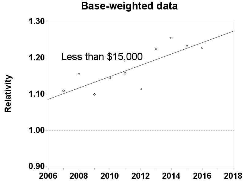
In the last two sections, we looked at the distributions of various socio-demographic characteristics among CE’s respondents relative to the ACS survey. The next two sections look at how those distributions changed over the ten-year period. The graphs show the ten-year period 2007-2016 on the horizontal axis, and the yearly “relativities” of selected socio-demographic characteristics on the vertical axis. Each graph also has a linear regression line showing how the relativities changed over time. Error: Reference source not found shows the following socio-demographic characteristics have statistically significant trends for one or more subgroups: age, CU size, monthly rent, and CU income.

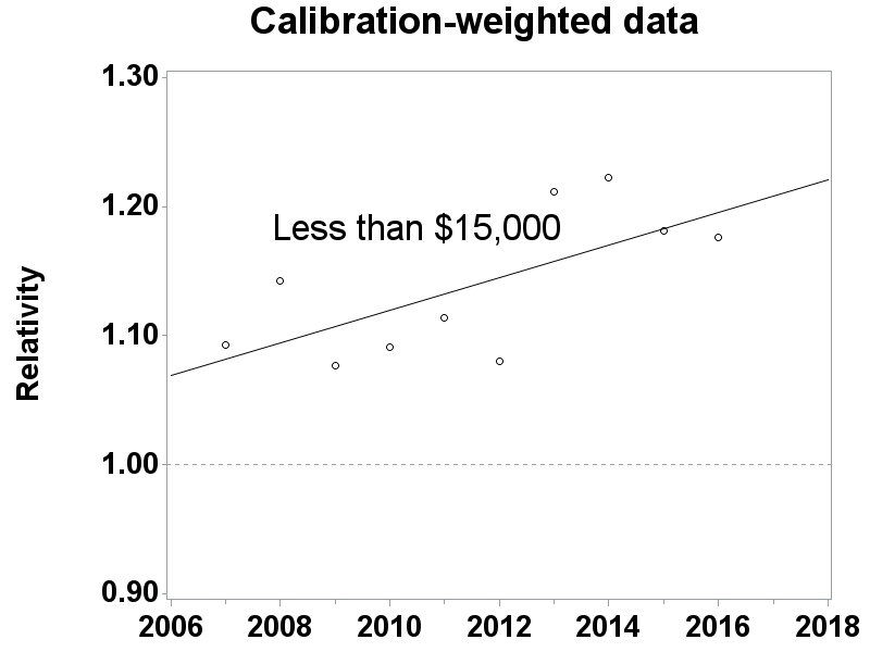
CU Income. The lower-income subgroups: less than $15,000, $15,000 to $24,999, and $25,000 to $34,999 have regression lines with statistically significant slopes. Their p-values were p=0.004, p=0.010, and p=0.002, respectively, for the base-weighted data. All three subgroups have regression lines that start between 1.06 and 1.11 and increase to between 1.20 and 1.25. That means CUs in these subgroups were over-represented by 6 percent to 11 percent relative to the ACS survey at the beginning of the ten-year period and they were over-represented by 20 percent to 25 percent at the end of the ten-year period. Since movement towards 1.00 is a good thing and movement away from 1.00 is a bad thing, these subgroups are moving in the wrong direction. The less than $15,000 subgroup is shown in the graph below.

CU Income in the CE Interview Survey lower income groups that are over-represented

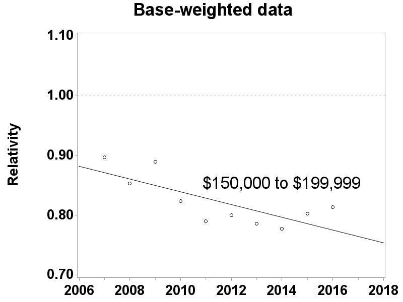
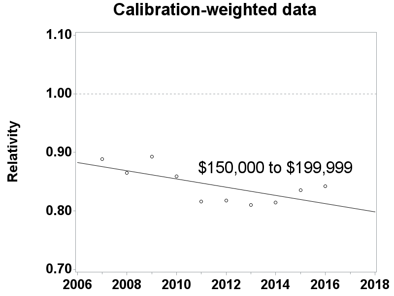
Three of the higher-income subgroups: $50,000 to $74,999, $150,000 to $199,999, and greater than $200,000 have regression lines that start below 1.00 and slope downward. Since movement towards 1.00 is a good thing and movement away from 1.00 is a bad thing, this is bad news for these subgroups. Moreover, the graphs for the base-weighted data and the calibration-weighted data are similar to each other, which shows that CE’s weighting procedures do not fix the problem. These results are consistent with other recent research findings that show high-income CUs are under-represented in the CE Interview survey and that CE’s weighting procedures do not fix the problem.¹² The $150,000 to $199,999 is shown below.

CU Income in the CE Interview Survey Higher income groups that are under-represented

Summary. The graphs in this section show two things: they show that the CE Interview survey and the ACS survey have different distributions for several socio-demographic characteristics, and they show that the relationships between some of those distributions are changing over time. Assuming ACS’s distributions are more accurate than CE’s distributions, both of these things suggest that the CE Interview survey’s data are not MCAR. Furthermore, the difference in the distribution of CU incomes between the two surveys is growing over time. Low-income CUs are over-represented in the CE Interview survey relative to the ACS survey and their over-representation is growing over time, and high-income CUs are under-represented in the CE Interview survey relative to the ACS survey and their under-representation is also growing over time. This is a concern since CE is a survey about money, and it may result in CE’s expenditure estimates being under-estimated, and with the under-estimation growing over time. This will be discussed later in the report.

3.1.4. Regression analysis for the Diary survey

Just like in the Interview survey, Error: Reference source not found shows the results of the regression analysis from 2007 to 2016 for all subgroups in the Diary survey, with statistically significant test results highlighted in gray. However, unlike the Interview survey, CU income is the only socio-demographic characteristic in the Diary survey with statistically significant trends for more than one of its subgroups and its slopes are consistent with the Interview survey.

3.2. Comparison of response rates across subgroups: General information

This study examined the response rates among socio-demographic subgroups that could be identified for both respondents and nonrespondents. Any differences between them indicate that the pattern of “missing-ness” is not independent of other variables, and therefore the missing data are not MCAR. As mentioned earlier, such comparisons are usually limited in scope because little is known about the nonrespondents since they do not respond to the survey, and consequently the variables examined for them are often limited to a small number of variables on the sampling frame and maybe a few other variables that data collectors are able to collect for every sample unit regardless of their participation in the survey. The subgroups analyzed were region of the country (Northeast, Midwest, South, West), “urbanicity” (urban, rural), PSU size class, housing tenure (owner or renter), and housing values for owners and renters.^¹³

Base-weighted response rates were calculated for these subgroups separately for both the Diary survey and the four waves of the Interview survey. As a reminder, base weights are the inverse of a sample address’s probability of selection. Base-weighted response rates answer the question “What percent of the survey’s target population do the respondents represent?” Base-weighted response rates are defined as the sum of base-weighted interviewed units divided by the sum of base-weighted interviewed units plus the Type A noninterviews units. Type A noninterviews occur when no interview is completed at an occupied eligible housing unit.

Base-weighted response rate =

where:

w_i= base weight for the i^th CU;
I_i = 1 if the i^th CU is a completed interview, and 0 otherwise; and
A_i = 1 if the i^th CU is a Type A noninterview, and 0 otherwise.

Ideally, the socio-demographic subgroups to which a CU belongs should be known for every CU in the sample since missing values may distort the analysis. However, occasionally they were not. Therefore, the analysis was restricted to CUs with no missing values.

3.2.1. Interview survey: Comparison of response rates across subgroups

Interview survey response rates were examined across socio-demographic subgroups for the ten-year period (2007-2016) and their results are summarized in Error: Reference source not found, , and Appendix H. Error: Reference source not found shows response rates for each subgroup and the nation by wave for 2016 only in an effort to keep the report more condensed. summarizes the test results from the Rao Scott chi-square tests for each of the subgroup comparisons by Wave 4 only also in an effort to keep the report more condensed. As an example, the subgroup comparisons for region include the Northeast vs. Midwest, Northeast vs. South, Northeast vs. West, South vs. West, Midwest vs. South, and Midwest vs. West. Appendix H shows response rate relativities for each of the subgroups relative to the nation by year and wave. As an example, the relativities calculated for region include the Northeast vs. Nation, Midwest vs. Nation, South vs. Nation, and West vs. Nation. The response rate relativities are then used to create the regression lines that determine significance of the slope. For each of the four interview waves, all possible pairs of subgroups within the six categories were examined over the ten-year period.

Using a level of significance α=0.05, a linear regression t-test is used to determine whether the slope of the ten point regression line (each point represents one year) differs from zero. For example, if the slope is 0.0038 (i.e., the response rate relativity increases 0.0038 per year) and the standard error of the slope is 0.0016, giving it a t-statistic of 2.38 (= (0.0038 – 0.0000)/0.0016), which means the slope is statistically different from zero at α=0.05 level of significance.

The two-way comparisons show that there are many statistical differences in response rates for every subgroup and since there is not a trend for convergence for the overwhelming majority of these comparisons, this strongly demonstrates that the data are not Missing Completely at Random for the Interview survey.

3.2.2. Diary survey: Comparison of response rates across subgroups

The Diary survey response rates analyses were examined across socio-demographic subgroups in a similar fashion to the Interview survey and their results are summarized in Error: Reference source not found, Error: Reference source not found, and Error: Reference source not found. Much like the Interview Survey, response rate differences within the subgroups suggest that the data are not MCAR because the respondent and nonrespondent CUs are not simple cross sections of the original sample.

3.3. Models for determining MCAR

As stated earlier, separate models were created for the Interview and Diary surveys using all ten years of data available for developing them. For the Interview survey, 383,054 observations were used and for the Diary survey, 201,122 observations were used. The dependent variable for the models were probability of response (yes/no) and the independent variables were the available candidates on the frame with both respondents and nonrespondents, all of which were categorical variables. These categorical variables were region of the country (Northeast, Midwest, South, West), “urbanicity” (urban, rural), PSU size class, housing tenure (owner or renter), and housing value quartiles for owners and renters. For each of these variables, a reference level was chosen and depending upon coding, either the user selects the reference level or SAS selects it by default as part of the regression procedures. Stepwise logistic regression with forward selection was the chosen method to create a model with good fit for both surveys, independently for these categorical variables. Once the iteration processes were completed, the main effects variables were chosen and all interaction terms using these variables were added and evaluated. The results for both survey models included the statistically significant variables, tenure, region, and urbanicity as the main effects and many of their two and three way interaction terms. There were only slight differences between the two models regarding interaction terms and both showed similar results using the Hosmer and Lemeshow Goodness-of-Fit Test^¹⁴. High p values, 0.6543 and 0.6671 from the test for the Interview and Diary models respectively confirmed that the data was a good fit for both models.

The successful creation of these models shows that there is a relationship between response and multiple socio-demographic variables confirming that the data are not MCAR. These models will be the foundation for calculation of nonresponse bias estimates for expenditures and are fully described in later in the report.

4. Calculating Relative Nonresponse Bias

4.1. OMB nonresponse bias equation

To estimate nonresponse bias, OMB (2006) provided a specific formula for computing the nonresponse bias of the respondent sample mean. This is given by:

where:

is the mean based on all sample cases;
is the mean based only on respondent cases;
is the mean based only on nonrespondent cases;
is the number of cases in the sample;
is the number of nonrespondent cases in the sample; and
is the nonresponse bias of the respondent sample mean.

Slight modifications to the nonresponse bias formula were necessary because relevant data (e.g., expenditures) were not available for the CE nonrespondents. After the modifications were made, the application of the formula to CE expenditure data becomes:

where:

is the base-weighted mean of expenditures for all CUs (this estimate includes all CUs, respondents and proxy nonrespondents);
is the base-weighted mean of expenditures for all respondent CUs (this estimate excludes proxy nonrespondents CUs from the calculation);
is the base-weighted mean of expenditures for all proxy nonrespondent CUs;
is the base-weighted number of CUs;
is the base-weighted number of proxy nonrespondent CUs; and
is the nonresponse bias in the base-weighted respondent sample mean.

Proxy nonrespondents are respondents with low contact rates. Their difficulty in being contacted makes them similar to nonrespondents in terms of their low probability of participating in the survey, and it is assumed that they are similar to nonrespondents in other ways as well, such as in the expenditures they make.

For the estimates of nonresponse bias in the proxy nonrespondent study, we computed relative nonresponse bias, instead of absolute nonresponse bias, as given in the formula above. The reason is that the dollar amounts vary substantially across expenditure categories, making comparisons difficult. Relative bias is a more appropriate statistic for comparisons across categories. The relative nonresponse bias is a percentage calculated by dividing the nonresponse bias by the adjusted base-weighted mean expenditures of all CUs and is shown below:

As a final point of clarification, the above formula was applied separately for each method. For Method 1, represents the base-weighted respondent mean and represents the FINLWT21 weighted respondent mean, for Methods 2 and 3, represents the base-weighted respondent mean and represents the Propensity-weighted respondent mean, and for Method 4, represents the weighted “pseudo respondent” mean and represents the all base-weighted respondents’ mean.

4.2. Variance estimation

Estimates of means were made using PROC SURVEYMEANS which is designed for complex sample surveys like CE. For variance calculations, the method of Balanced Repeated Replications (BRR using Fay technique) was chosen as opposed to simple random sampling or random groups since they understate the variance for Non-self-representing (“N” and “R”) PSUs. This is due to it measuring the “within-PSU” portion of the variance but not the “between - PSU” portion of the variance. BRR does account for the portion of the variance caused by PSU “X” being selected for the sample instead of PSU “Y” while other simpler methods do not. As stated above, the variance formula used PROC SURVEYMEANS for all four methods where the assigned half sample represents the cluster variable and the row of the matrix represents the strata variable in the formula.

4.3. Significance tests

A 95 percent confidence interval of the relative nonresponse bias of expenditures was computed for each expenditure variable. Calculations were performed by year and wave for the selected Interview survey variables and individually by method. If the confidence interval excludes zero then that test is considered significant and there would be a bias. If the confidence interval is entirely negative then the relative bias is considered negative while if the interval is entirely positive then the relative bias is considered positive. For the Diary survey, there are no waves so only the year was analyzed for relative bias.

For the Interview survey, ten individual years of data were analyzed per wave in this study (2007-2016), with a separate analysis done for each selected variable individually by method. That means ten 95 percent confidence intervals, with one statistic generated for each wave by year, and the results were summarized by counting the number of times statistically significant results were obtained. If the confidence interval showed positive bias, then it was given a score of “+1”; if it showed negative bias, then it was given a score of “–1”; and if there was no bias it was given a score of “0.” After summing by wave, the relative bias for each variable was then categorized as “strongly positive” if the overall score was greater than or equal to +5 and “strongly negative” if less than or equal to –5; “moderately positive” if equal to +3 or +4 and “moderately negative” if –3 or –4; and “not significantly biased” if it was between –2 and +2. This is comparable to the two-way socio-demographic variable comparisons discussed earlier in the report.

In a similar manner, four waves of data were analyzed per year in this study (Waves 1-4) and a similar scoring system was developed. That means four 95 percent confidence intervals, with one statistic generated for each wave by year, and the results were summarized by counting the number of times statistically significant results were obtained. Similar to above, if the confidence interval showed positive relative bias, then it was given a score of “+1”; if it showed negative relative bias, then it was given a score of “–1”; and if there was no bias it was given a score of “0.” Then the four scores for each of the ten years were summed by wave, giving an overall possible score between –4 and +4 for each wave. The relative bias for each year for each variable was then categorized as “strongly positive” if the overall score was +3 or +4 and “strongly negative” if -3 or -4, “moderately positive” if it was +2 and “moderately negative” if –2; and “not significantly biased” if it was between –1 and +1. The results for these calculations are summarized on Appendix M.

The Diary survey does not have waves, each of the ten years were summarized using similar logic to the Interview survey discussed above. If the confidence interval showed positive bias, then it was given a score of “+1”; if it showed negative bias, then it was given a score of “–1”; and if there was no bias it was given a score of “0.” These results are summarized in Appendix O.

5. Description of the Four Methods Used in Calculation of Relative Bias

The following four methods were used to measure presence of nonresponse bias in the data in the CE sample. Each method has its strengths and weaknesses and there was no correct or incorrect method. The main goal of having multiple methods was to develop a range of results for each selected expenditure category to help determine whether nonresponse bias exists in the CE surveys and if it is increasing over time or by wave. All of the relative bias methods in this report use base weights and Method 1 also used the final calibration weights.

5.1. Method 1

Method 1 calculates bias as the difference between the weighted estimate of the population mean prior to any nonresponse adjustment minus the estimate that considers all nonparticipation of which nonresponse is the largest component. This estimate assumes that response is MAR and response correction of FINLWT21 is a reasonable estimate to the inverse of the response probability. This method uses the general bias formula, , where is weighted estimate of the population mean expenditure ignoring response, is the base-weight and R denotes the set of the respondents. can be estimated by , and can be estimated by a reasonable estimate that takes into account non participation and more specifically, nonresponse. Assuming that the FINLWT21 weighted estimate accounts for nonresponse, can be estimated by , where is the FINLWT21 weight. This estimate assumes that response is MAR and response correction to the FINLWT21 weight is a reasonable estimate to the inverse of the response probability. Therefore, the nonresponse bias can be estimated by

where where is the base-weighted mean and is the FINLWT21 weighted mean.

5.2. Method 2

Method 2 calculates the difference between the weighted estimates of the population mean ignoring response minus the propensity-weighted estimate that assumes nonresponse is a reasonable estimate of probability to respond. This propensity-weighted estimate is developed using a logistic regression model that contains socio-demographic variables. In the first nonresponse bias report released earlier this year, it was determined that the surveys’ response rates are affected by certain socio-demographic variables. Those variables were household tenure, urbanicity, region of the country and many of their two-way interaction terms. Further research showed that CU size was also a good variable to use and was added to the model.

The selected Interview survey model was:

( = + I(Rural) + (Renter) + I(Tenure Other) + (Midwest) + (South) + (West) + (CU Size 1) + (CU Size 2) + (CU Size 3 or 4) + (Percentage of Noncontacts) + + (CU Size 1*Rural) + (CU Size 2*Rural) + (CU Size 3 or 4 * Rural) + (CU Size 1 * Renter) + (CU Size 1 * Tenure Other) + (CU Size 2 * Renter) + (CU Size 2 * Tenure Other) + (CU Size 3 or 4 * Renter) + (CU Size 3 or 4 * Tenure Other) + (CU Size 1 * Midwest) + (CU Size 1 * South) + (CU Size 1 * West) + (CU Size 2 * Midwest) + (CU Size 2 * South) + (CU Size 2 * West) + (CU Size 3 or 4 * Midwest) + (CU Size 3 or 4 * South) + (CU Size 3 or 4 * West) where is the probability of response.

The Interview survey and Diary survey have similar models with the only difference being several interaction terms involving Tenure*Region, Tenure*Urban, and CU Size*Urban which were included in the Interview survey model but not the Diary survey model.

As a reminder, logistic regression is a model of the outcomes of a binary process, such as whether a sample household participates in the CE survey. It has a specific algebraic form that ensures its numeric values are between 0 and 1, which makes it suitable for modeling probabilities:

Simple algebra allows the model to be rewritten like this:

To estimate nonresponse bias, Method 2 estimates by the estimate of the CU’s probability of responding:

, where

is the estimate of the CU’s response probability (propensity score), assuming that the non-response is MAR and is a reasonable estimate of probability to respond. The resulting propensity scores will have a score between 0 and 1.0 and the reciprocal of this propensity will be multiplied by the current base-weight to get the adjusted base-weight. Relative bias can then be estimated by where is the base-weighted mean and is the propensity adjusted base-weighted mean.

One of the main goals of this research was to determine if changing response rates over time had an impact on the magnitude of nonresponse bias. There were significant drops in response rates for both the Interview and Diary surveys over the research period and so it was decided to treat each year separately when determining propensity scores. Therefore, each year was its own model when calculating propensity scores.

5.3. Method 3

Method 3 is nearly identical to Method 2 except that it contains a contact history variable (noncontact percentage) in the logistic regression model in addition to all of the socio-demographic variables discussed in Method 2. This contact history variable was calculated as the percent of noncontacts during the interview process and was determined to have a strong relationship to response. A small percentage of data, 1.4 percent of all CUs from the Interview survey, did not have contact history (CHI) data so these CUs were removed from the logistic regression model when calculating the propensity scores. Only 0.5 percent of these CUs were responders and since they did not have propensity scores they were not included in the calculation of relative bias. The Diary survey had even fewer CUs (0.9 percent) with missing CHI data, and only 0.4 percent of the responders had missing CHI data. Everything else pertaining to Method 2 described above also applied to Method 3.

5.4. Method 4

For Method 4, responders were divided into proxy responders and proxy nonresponders based on contact history. Responders that have high contact rates were treated as proxy “pseudo” responders while those with low contact rates were treated as proxy “pseudo” nonresponders since they were harder-to-contact. It assumes that the “pseudo nonresponders” from the real respondent part of the sample behave like real nonrespondents regarding expenditure patterns. This assumption is almost uncheckable but is based on the theory known as the continuum of resistance to identify certain respondents to serve as proxy nonrespondents. The theory suggests that sampling units can be ordered by the amount of interviewer effort needed in order to obtain a completed interview (Groves, 2006) and was used in the previous nonresponse bias study.^¹⁵

Using data collected in the Interview survey Contact History Instrument (CHI), respondents were defined to be “harder to contact” when greater than 50 percent of the contact attempts resulted in noncontacts. The only exception was if there were two contact attempts resulting in one contact, these CUs were not considered “harder to contact” and were treated as pseudo responders. This cut-off was selected to yield a response rate that coincided with the observed response rates during the ten-year period covered by the data that ranged from the lower 60’s percent to lower 70’s percent.

The formula used to calculate the relative bias was similar to those mentioned above except the numerator is the difference between the base-weighted mean of the pseudo respondents and the base-weighted mean of all respondents divided by the base-weighted mean of all respondents. It can be shown as follows:

Where:

5.5. Results Using the Four Methods Used in Calculation of Relative Bias

5.5.1. Interview Survey Variables Analyzed

The main variable to be discussed is the summary variable, ZTOTALX4 that contains all CE Interview expenditures. The five largest summary variables based on expenditures are also analyzed individually and they include; ZHOUSING (housing expenditures), ZTRANPRT (transportation expenditures), ZFOODTOT (food expenditures), ZPERLINS (personal insurance expenditures), and ZHEALTH (health expenditures). These variables are defined in more detail in Appendix A. In addition, eight of the smaller expenditure summary variables were added together into a variable called Z_EIGHT and were analyzed as a group. Z_EIGHT consists of summary variables for alcoholic beverages, apparel, cash contributions, education, entertainment, personal care, reading materials, and tobacco.

As has been discussed, four methods to estimate relative nonresponse bias were used in the analysis. For some of the summary variables there were similar levels of nonresponse bias with a fairly narrow range of estimates. The summary variables were analyzed by year to determine if relative bias has changed over time and by wave to determine if different interview waves contain more or less bias than others. As described earlier in the report, relative nonresponse bias point estimates are a percentage calculated by dividing the nonresponse bias by the adjusted base-weighted mean expenditures of all CUs. These point estimates of relative bias are displayed on every graph and when analyzed in conjunction with their standard errors a determination of significance was made.

There are consistent patterns in the standard errors between the four methods that play a major role in determining significance. Method 2 contains the smallest standard errors followed by Method 1, then Method 3 and finally Method 4. The only difference between the models for Method 2 and Method 3 is the inclusion of the percent of noncontacts variable in Method 3. This is the major cause for the wider range in propensity scores and subsequently a wider range of adjusted base-weights and larger standard errors between these two methods. Similar relative bias expenditure means can easily result in much different levels of significance when the standard errors differ greatly

5.5.2. Interview Survey Findings

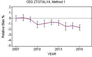
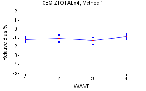
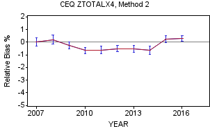
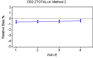
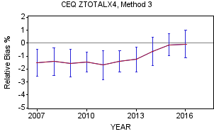
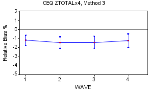
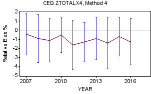
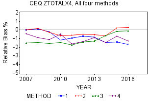
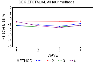
ZTOTALX4 by Year

The graphs for Methods 1-3 show negative relative bias for all three methods for years 2010-2013 while there are varying degrees of negative relative bias for the earlier years and in later years of the research period. In fact, Method 2 for 2016 actually shows a positive bias. In general, the three methods have relative bias means ranging from around -1.7 percent to around 0.3 percent with confidence intervals ranging from around -2.8 percent to just below 1.0 percent. Over the ten-year period, the trend in the relative bias of the means show a negative trend for Method 1, a U-shaped pattern for Method 2 and a bit of an upward trend for Method 3. The graphs above for Methods 1-3 indicate significance for years where the 95 percent confidence intervals do not include zero.

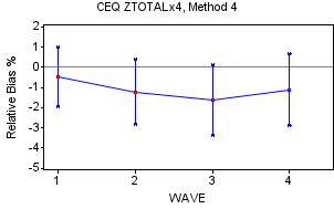
Method 4 has comparable means to the other three methods but has by far the largest standard errors. Because their large standard errors result in wide confidence intervals, there are no years where the relative bias is statistically significant for ZTOTALX4 as shown on their graph below. This is consistent with the results from the previous report’s research using this method on 2005-2006 data. Over the ten-year period, ZTOTALX4 has shown moderate to strong negative bias when summing over the waves, with scores frequently totaling between -2 and -4 with possible values between -4 and +4. This is shown on the left hand side of Appendix M and Methods 1-3 all show this type of result.

The graph that summarizes the relative bias means for all four methods by year do not differ that dramatically. It contains each of the four methods from the graphs above without the confidence intervals. They are within one percentage point of each other for the middle years of the research period, 2010-2014, and overall slightly negative throughout the ten-year period. This slight negative relative bias implies that our responders spend a little less than our nonresponders (after adjusting for nonresponse in Methods 1-3) when evaluating by year. Method 4, which separates the responders into pseudo responders and pseudo nonresponders (described earlier), shows similar results. Overall, the graph shows that there is not total agreement regarding a recent relative bias trend where two of the methods (Method 2 and Method 3) have trended slightly positive while Methods 1 and 4 have trended more negative. In addition, through 2013, Method 1 and Method 2 were similar but split beginning in 2014 with Method 1 showing close to -1.5 percent and Method 2 just above 0 percent.

ZTOTALX4 by Wave

The 95 percent confidence intervals show the presence of negative relative bias for all waves for ZTOTALX4 for Methods 1-3. The results on Appendix N quantify this for Methods 1-3 having scores between -8 and -4 implying moderate to strong significant presence of negative relative bias over the ten-year period. Reinforcing the earlier statement, Method 4 shows no relative bias in either direction that are likely due to large standard errors by wave. All of this can be seen on the individual graphs by method, above. There is some evidence that ZTOTALX4 expenditures for Wave 4 display slightly less negative relative bias than the other waves for most of the methods. The graphs above show Wave 4 with the lowest or next to the lowest relative bias values when viewing the four methods. Perhaps, this is due to an extra effort by the field reps to get the CUs to participate in the survey. In addition, Appendix N shows that Methods 1-3 contain moderate to strong presence of negative relative bias by wave. Appendix N also shows that Method 4 does not have significant negative bias even though its mean values are comparable to the other three methods due to larger standard errors.

Other Interview Survey Summary Variables

The results of the majority of these summary variables (ZHOUSING, ZPERLINS, ZTRANPRT, ZFOODTOT, Z_EIGHT, and ZHEALTH) are comparable to ZOTALX4 regarding relative bias with the exception of ZHEALTH whose estimates are more widespread. Specifically, ZHOUSING, which comprises about 33 percent of all Interview Survey expenditures, Z_EIGHT (15 percent) and ZPERLINS (11 percent of expenditures), have similar patterns especially regarding Methods 1-3. Their results are shown in Appendix M and Appendix N.

Interview Survey Summary

In summary, the four methods for the Interview survey show the presence of slight negative relative bias over time and by wave when analyzing several of the summary variables, especially ZTOTALX4, ZHOUSING, ZPERLINS, ZTRANPRT, ZFOODTOT, and Z_EIGHT. The level of negative relative bias is generally in the range of -0.5 percent to -1.5 percent and varies somewhat by method but does not appear to be strongly correlated to the decreasing response rates over the ten-year period. As mentioned earlier, there is a pattern showing the Wave 4 relative bias being slightly less than the other waves. ZHEALTH behaves a bit differently than the other summary variables with more positive relative bias values, especially for Method 4.

5.5.3. Diary Survey Variables Analyzed

Similar to the Interview survey, four methods to estimate relative bias were used in the Diary survey analysis. There were five summary variables analyzed; ZTOTAL (total expenditures), Z_FDB (expenditures of food for home consumption), Z_MLS (expenditure of meals purchased away from home), Z_CLO (expenditures of clothing purchased), and Z_OTH (total of all other items purchased). The summary variables were analyzed by year to determine if bias has changed over time. Since Z_OTH represents nearly 80 percent of the ZTOTAL expenditures, only ZTOTAL is discussed but the other summary variables are covered in Appendix O.

The relative bias for the Diary survey using Methods 1-3 was calculated in the exact same manner as their Interview survey counterparts. There was one substantial difference between the Diary survey and Interview survey for calculating relative bias using Method 4. For the Diary survey, a noncontact percentage greater than 45 percent was used as the cut-off to determine pseudo responders versus pseudo nonresponders. This was the percentage required to yield a response rate ranging from the upper 50’s percent to the middle 70’s percent during the ten-year period. The previous report, (approximately 10 years ago) which analyzed only the Interview survey also chose 45 percent as its cut-off.

5.5.4. Diary Survey Findings

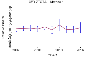
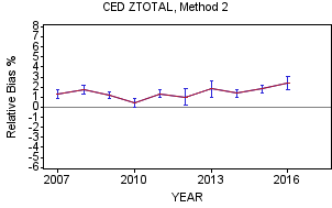
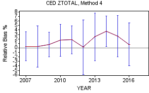
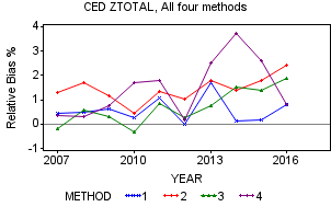
ZTOTAL

The four methods for ZTOTAL, the Diary survey summary variable that contains all expenditures, show a positive relative bias in the range of 0.5 percent to 2.0 percent over the ten-year period. On the graphs above, Methods 2 and 3 show slight indications of upward movement in positive relative bias in the more recent several years while Method 1 and Method 4 do not.

In similar fashion to the Interview survey, each of the four methods for ZTOTAL have a graph with 95 percent confidence intervals for each year to determine statistical significance. In general, the confidence intervals are wider than the Interview survey due to larger standard errors resulting from smaller number of CUs (approximately half) which has the potential to make it more difficult to obtain statistical significance. This pattern exists for all the methods but is especially true for Method 4 and these confidence intervals are shown in the graphs above.

However, the four methods vary greatly regarding the level of statistical significance over the period. As shown on Appendix O, Methods 1 and 4 each have only one out of the 10 years showing significant positive relative bias while all ten years for Method 2 show significant positive relative bias. Method 3 is in the middle where four of the ten year show significant positive relative bias.

In summary, the four methods shows the general widespread 0.5 percent to 2.0 percent, positive bias with only a few years having a slight negative relative bias and one outlier with a high positive bias (Method 4, 2014). As a reminder, a slight positive relative bias implies that CE responders are spending a little more than the estimates for nonresponders, which is opposite compared to most summary variables in the Interview survey.

Diary Survey Summary

In summary, there is a slight level of positive relative bias for most of the summary variables in the Diary survey including the all expenditures variable, ZTOTAL. The estimates produced by the methods do vary from year to year with Method 2 showing the most occurrences of statistically significant positive relative bias for each of the summary variables shown on Appendix O. When looking at the ZTOTAL graph, the four methods hint at a slight trend towards increasing positive bias but not as dramatically as the drop in Diary survey response rates over the ten-year period. A strong correlation that would show increasing nonresponse relative bias, either positive or negative, related to declining response rates could be cause for concern. A reminder that positive relative nonresponse bias is not a measure of respondents underreporting expenditures but instead compares the responders’ actual reported expenditures to the four estimates of the nonresponders’ reported expenditures.

6. Conclusion

In 2006, OMB issued a directive requiring any federal household survey with a response rate below 80 percent to perform a nonresponse analysis. Both the Interview and Diary surveys have a response rate below 80 percent. Each of the four studies in this report was designed to analyze nonresponse in the Interview and Diary surveys by answering one or more of the following questions: (1) Are the data in the Interview and Diary surveys MCAR? (2) What are the demographic characteristics of the nonrespondents and respondents? and (3) What additional information does the linear trend analysis provide regarding socio-demographic movement over the ten collection years?

Statistically significant differences were found by region of the country, PSU size class, urbanicity, and housing tenure for the Interview survey and for all subgroups except Housing value for the Diary survey. Likewise, the study comparing respondent demographic characteristics to the American Community Survey’s population found statistically significant differences for most of the variables examined. Because statistically significant differences were found in each of these studies, we conclude that the data are not MCAR. No individual analysis was intended to provide a definitive answer to the questions raised in this research. However, they all conclude that the Interview and Diary survey respondents and nonrespondents have different characteristics for many variables and the data are not MCAR.

The second part of the report analyzes the results of four methods undertaken with ten years of data to respond to OMB’s directive about determining the amount of nonresponse bias in the CE Interview and Diary Surveys. Since the first report concluded that the missing data for both surveys were not MCAR, the concern involved the commonly held belief that the nonrespondent’s missing data were vulnerable to nonresponse bias. From the OMB equation, the nonresponse bias will be zero if the mean expenditure for respondents is equivalent to the mean expenditures for nonrespondents.

The total expenditure summary variable for the Interview survey, ZTOTALX4, was analyzed in detail to determine if there was a presence of relative nonresponse bias. Analysis of the Interview survey presented robust graphic detail and tables of bias for ZTOTALX4 by year and wave. The results showed a slight negative relative bias in a general -0.5 percent to -1.5 percent range over the ten-year period. This implies that the responders spent a little less than the nonresponders over the period and there was statistical evidence supporting this.

The Diary survey total expenditures summary variable, ZTOTAL, was also analyzed in detail to determine if there was a presence of relative nonresponse bias. As opposed to the total expenditures variable in the Interview survey, this variable showed a slight positive relative bias in a general 0.5 percent to 2 percent range over the ten-year period. This implies that the responders spent a little more than the nonresponders over the period.

None of the four methods was designed to exclusively determine the exact level of relative bias but rather provide a range of estimates. Each method had its strengths and weaknesses and they differ enough to provide a realistic range of estimates for the analysis. Under the MAR assumption, the conclusion is that the relative bias seems to be minor and not essentially important.

Appendices

Appendix A

Interview survey 2016 – Comparison of selected characteristics of CE respondents to the ACS

		CE Interview survey					CE Interview survey
	ACS	Base-Weighted	Noninterview-Weighted	Calibration-Weighted		ACS	Base-Weighted	Noninterview-Weighted	Calibration-Weighted
Gender (%)^1,2,3					Number of rooms in housing unit (%)^1,2,3
Male	49.2	48.6	48.5	48.6	1	2.4	1.5	1.8	1.6
Female	50.8	51.4	51.5	51.4	2	2.7	2.5	2.5	2.4
Age (%)^1,2					3-4	25.6	23.6	24.0	23.2
Under age 25	32.4	31.9	30.9	32.5	5-6	37.7	38.2	37.9	38.1
25-34	13.7	12.5	12.7	13.7	7-8	20.6	24.0	23.8	24.3
35-44	12.6	12.4	12.4	12.5	9 +	11.1	10.1	10.0	10.3
45-54	13.2	13.0	13.2	13.3	Owner-occupied housing value (%)^1,2,3
55-64	12.8	13.5	13.8	13.0	Less than $50,000	7.3	7.3	7.2	7.2
65-74	8.9	9.8	10.1	8.9	$50,000 to $99,999	13.1	13.8	13.7	13.6
75 and over	6.4	6.8	6.9	6.1	$100,000 to $149,999	14.1	14.4	14.2	14.2
Race (%) ^1,2,3					$150,000 to $199,999	14.5	15.6	15.5	15.5
White	72.6	81.1	81.0	79.5	$200,000 to $299,999	19.2	19.2	19.1	19.2
Black	12.7	11.3	11.4	12.9	$300,000 to $499,999	18.2	18.0	18.2	18.3
Other	14.7	7.6	7.6	7.5	$500,000 to $999,999	10.5	9.2	9.4	9.4
Education* (%)^1,2,3					$1,000,000 +	3.1	2.5	2.6	2.6
Less than high school	12.5	12.5	12.2	12.1	Monthly rent (%)^1,2,3
High school graduate	27.2	26.7	26.6	26.6	Less than $500	16.8	20.7	20.6	19.8
Some college/Assoc degree	29.0	27.9	27.8	27.9	$500 to $749	22.7	23.4	23.3	23.1
College graduate	31.3	32.9	33.5	33.4	$750 to $999	20.1	20.5	20.5	20.9
CU size (%)^1,2,3					$1,000 to $1,499	20.8	19.7	19.7	20.3
1 person	28.0	30.9	32.1	29.6	$1,500 to $1,999	8.5	7.0	7.1	7.4
2 persons	33.9	33.2	33.9	33.0	$2000 +	6.0	5.6	5.7	5.6
3 persons	15.6	14.6	14.1	15.0	No cash rent	5.0	3.0	2.9	2.9
4+ persons	22.5	21.3	19.9	22.4	CU income (%)^1,2,3
Housing tenure (%)^1,2,3					Less than $15,000	11.5	14.1	14.4	13.5
Owner	63.1	62.1	61.7	62.3	$15,000 to $24,999	9.7	12.6	12.7	12.1
Renter	36.9	37.9	38.3	37.7	$25,000 to $34,999	9.5	11.3	11.3	11.1
					$35,000 to $49,999	13.0	13.4	13.3	13.3
					$50,000 to $74,999	17.7	15.7	15.6	15.8
					$75,000 to $99,999	12.3	10.9	10.9	11.3
					$100,000 to $149,999	14.0	11.9	11.9	12.4
					$150,000 to $199,999	5.8	4.7	4.7	4.9
					$200,000 +	6.4	5.3	5.3	5.5

^{1, 2, 3} Indicates a statistically significant difference (p < 0.05) between the ACS and the Interview survey, where “1” is for the base-weighted results, “2” is for the noninterview-weighted results, and “3” is for the calibration-weighted results.

* Comparison for persons age 25 and older

Appendix B

Comparison of CE’s and ACS’s demographic distributions over the 10-year period 2007–2016:

The number of years the Rao-Scott chi-square statistic showed a statistically significant difference between CE and ACS (p<0.05) for both the Interview and Diary surveys

Interview survey:

Demographic characteristic	Base-weighted CE data vs. ACS	Noninterview-weighted CE data vs. ACS	Calibration-weighted CE data vs. ACS
Gender	10	10	10
Age	10	10	4
Race	10	10	10
Education	10	10	10
CU size	10	10	10
Tenure	6	9	1
# Rooms in housing unit	10	10	10
Owner-occupied housing value	10	10	10
Monthly rent	10	10	10
CU income	10	10	10

Diary survey:

Demographic characteristic	Base-weighted CE data vs. ACS	Noninterview-weighted CE data vs. ACS	Calibration-weighted CE data vs. ACS
Gender	5	5	4
Age	10	10	0
Race	10	10	10
Education	10	10	10
CU size	10	10	6
Tenure	7	1	0
CU Income	10	10	10

Appendix C

Interview survey: Relativity regression results for CE to ACS comparison of subgroups

	CE subgroup percentage / ACS subgroup percentage
	Base-weighted		Noninterview-weighted		Calibration-weighted
Subgroup*	P-value	Slope	P-value	Slope	P-value	Slope
Gender
Male	0.035	Positive	0.072	Positive	0.079	Positive
Female	0.034	Negative	0.071	Negative	0.078	Negative
Age
Under age 25	0.010	Negative	0.004	Negative	0.786	Positive
25-34	0.661	Negative	0.762	Positive	0.061	Negative
35-44	0.512	Positive	0.594	Positive	0.426	Negative
45-54	0.308	Negative	0.532	Negative	0.456	Negative
55-64	0.919	Negative	0.395	Negative	0.730	Negative
65-74	0.005	Positive	0.018	Positive	0.386	Positive
75 and over	0.098	Positive	0.571	Positive	0.001	Positive
Race
White	0.507	Positive	0.524	Negative	0.688	Positive
Black	0.405	Negative	0.020	Positive	0.339	Negative
Other	0.090	Positive	0.112	Positive	0.114	Positive
Education
Less than high school	0.114	Negative	0.036	Negative	0.057	Negative
High school graduate	0.214	Positive	0.336	Positive	0.201	Positive
Some college/Assoc degree	0.645	Negative	0.620	Negative	0.538	Negative
College graduate	0.425	Positive	0.027	Positive	0.150	Positive
CU size
1 person	0.017	Positive	0.001	Positive	0.788	Negative
2 persons	0.982	Positive	0.700	Positive	0.811	Positive
3 persons	0.605	Positive	0.966	Positive	0.254	Positive
4+ persons	0.001	Negative	0.000	Negative	0.354	Negative
Housing tenure
Owner	0.180	Negative	0.015	Negative	0.203	Negative
Renter	0.207	Positive	0.009	Positive	0.239	Positive
Number of Rooms
1	0.595	Negative	0.794	Negative	0.608	Negative
2	0.075	Positive	0.044	Positive	0.176	Positive
3-4	0.019	Positive	0.008	Positive	0.099	Positive
5-6	0.190	Positive	0.466	Positive	0.323	Positive
7-8	0.068	Negative	0.016	Negative	0.190	Negative
9 +	0.020	Negative	0.020	Negative	0.048	Negative

* Shaded data in this table show the subgroups where the β₁ coefficient is significant, as well as the direction of the slope for the ten-year regression line.

Interview survey: Relativity regression results for CE to ACS comparison of subgroups -- Continued

	CE subgroup percentage / ACS subgroup percentage
	Base-weighted		Noninterview-weighted		Calibration-weighted
Subgroup*	P-value	Slope	P-value	Slope	P-value	Slope
Owner-occupied housing value
Less than $50,000	0.732	Positive	0.888	Positive	0.950	Positive
$50,000 to $99,999	0.067	Positive	0.093	Positive	0.140	Positive
$100,000 to $149,999	0.112	Positive	0.104	Positive	0.168	Positive
$150,000 to $199,999	0.889	Negative	0.858	Negative	0.873	Negative
$200,000 to $299,999	0.093	Negative	0.118	Negative	0.136	Negative
$300,000 to $499,999	0.254	Negative	0.299	Negative	0.418	Negative
$500,000 to $999,999	0.375	Negative	0.500	Negative	0.766	Negative
$1,000,000 +	0.856	Positive	0.725	Positive	0.549	Positive
Monthly rent
Less than $500	0.988	Negative	0.868	Positive	0.377	Negative
$500 to $749	0.088	Positive	0.090	Positive	0.192	Positive
$750 to $999	0.050	Positive	0.088	Positive	0.046	Positive
$1,000 to $1,499	0.033	Positive	0.095	Positive	0.066	Positive
$1,500 to $1,999	0.599	Negative	0.556	Negative	0.923	Negative
$2000 +	0.608	Negative	0.696	Negative	0.998	Positive
No cash rent	0.151	Positive	0.174	Positive	0.178	Positive
CU income
Less than $15,000	0.004	Positive	0.002	Positive	0.029	Positive
$15,000 to $24,999	0.010	Positive	0.020	Positive	0.041	Positive
$25,000 to $34,999	0.002	Positive	0.002	Positive	0.005	Positive
$35,000 to $49,999	0.454	Negative	0.323	Negative	0.175	Negative
$50,000 to $74,999	0.024	Negative	0.023	Negative	0.044	Negative
$75,000 to $99,999	0.591	Negative	0.485	Negative	0.980	Negative
$100,000 to $149,999	0.206	Negative	0.153	Negative	0.789	Negative
$150,000 to $199,999	0.011	Negative	0.002	Negative	0.027	Negative
$ 200,000 +	0.288	Negative	0.300	Negative	0.952	Negative

* Shaded data in this table show the subgroups where the β₁ coefficient is significant, as well as the direction of the slope for the ten-year regression line.

Appendix D

Diary survey 2016 – Comparison of selected characteristics of CE respondents to the ACS

		CE Diary survey					CE Diary survey
	ACS	Base-Weighted	Noninterview-Weighted	Calibration-Weighted		ACS	Base-Weighted	Noninterview-Weighted	Calibration-Weighted
Gender (%)^1,2					CU income (%)^1,2,3
Male	49.2	48.5	48.6	48.7	Less than $15,000	11.5	12.5	12.7	12.4
Female	50.8	51.5	51.4	51.3	$15,000 to $24,999	9.7	12.2	12.3	11.8
Age (%)^1,2					$25,000 to $34,999	9.5	11.4	11.5	11.4
Under age 25	32.4	31.3	30.5	32.5	$35,000 to $49,999	13.0	14.3	14.3	14.3
25-34	13.7	12.3	12.4	13.7	$50,000 to $74,999	17.7	16.3	16.3	16.7
35-44	12.6	12.7	12.5	12.5	$75,000 to $99,999	12.3	11.5	11.5	11.9
45-54	13.2	13.7	13.9	13.3	$100,000 to $149,999	14.0	12.1	11.8	12.0
55-64	12.8	13.4	13.7	13.0	$150,000 to $199,999	5.8	5.1	5.0	5.1
65-74	8.9	9.9	10.2	8.9	$200,000 +	6.4	4.7	4.5	4.5
75 and over	6.4	6.6	6.8	6.2
Race (%) ^1,2,3
White	72.6	81.5	81.6	78.7
Black	12.7	10.0	10.1	13.1
Other	14.7	8.5	8.3	8.3
Education* (%)^1,2,3
Less than high school	12.5	11.5	11.4	11.5
High school graduate	27.2	25.5	25.6	25.4
Some college/Assoc degree	29.0	28.4	28.5	28.7
College graduate	31.3	34.6	34.6	34.4
CU size (%)^1,2
1 person	28.0	30.0	30.9	28.6
2 persons	33.9	34.1	34.8	33.9
3 persons	15.6	15.4	14.9	15.9
4+ persons	22.5	20.4	19.4	21.6
Housing tenure (%)
Owner	63.1	63.5	63.3	62.3
Renter	36.9	36.5	36.7	37.7

* Comparison for persons age 25 and older.

Appendix E

Diary survey – Relativity regression results for CE to ACS comparison of subgroups

	CE subgroup percentage / ACS subgroup percentage
	Base-weighted		Noninterview-weighted		Calibration-weighted
Subgroup*	P-value	Slope	P-value	Slope	P-value	Slope
Gender
Male	0.588	Positive	0.365	Positive	0.323	Positive
Female	0.584	Negative	0.362	Negative	0.319	Negative
Age
Under age 25	0.555	Negative	0.911	Negative	0.769	Positive
25-34	0.756	Negative	0.543	Negative	0.059	Negative
35-44	0.998	Negative	0.757	Positive	0.489	Negative
45-54	0.810	Negative	0.899	Negative	0.486	Negative
55-64	0.208	Negative	0.106	Negative	0.771	Positive
65-74	0.827	Positive	0.805	Negative	0.418	Positive
75 and over	0.043	Positive	0.107	Positive	0.000	Positive
Race
White	0.910	Negative	0.558	Negative	0.146	Negative
Black	0.448	Negative	0.532	Positive	0.043	Positive
Other	0.000	Positive	0.000	Positive	0.000	Positive
Education
Less than high school	0.378	Positive	0.446	Positive	0.361	Positive
High school graduate	0.152	Negative	0.133	Negative	0.124	Negative
Some college/Assoc degree	0.428	Negative	0.553	Negative	0.482	Negative
College graduate	0.359	Positive	0.352	Positive	0.352	Positive
CU size
1 person	0.137	Positive	0.807	Negative	0.065	Negative
2 persons	0.257	Negative	0.405	Negative	0.625	Positive
3 persons	0.335	Positive	0.220	Positive	0.075	Positive
4+ persons	0.251	Negative	0.632	Negative	0.461	Negative
Housing tenure
Owner	0.335	Negative	0.451	Positive	0.413	Negative
Renter	0.219	Positive	0.455	Negative	0.456	Positive
CU income
Less than $15,000	0.056	Positive	0.131	Positive	0.109	Positive
$15,000 to $24,999	0.004	Positive	0.009	Positive	0.033	Positive
$25,000 to $34,999	0.056	Positive	0.077	Positive	0.128	Positive
$35,000 to $49,999	0.395	Negative	0.361	Negative	0.490	Negative
$50,000 to $74,999	0.022	Negative	0.031	Negative	0.034	Negative
$75,000 to $99,999	0.167	Negative	0.501	Negative	0.781	Negative
$100,000 to $149,999	0.374	Negative	0.677	Negative	0.691	Negative
$150,000 to $199,999	0.862	Positive	0.795	Positive	0.757	Positive
$200,000 +	0.439	Positive	0.396	Positive	0.439	Positive

* Shaded data in this table show the subgroups where the β₁ coefficient is significant, as well as the direction of the slope for the ten-year regression line.

Appendix F

Interview survey 2016 – Subgroup response rates by wave

	Wave 1		Wave 2		Wave 3		Wave 4
Subgroup	n	Weighted Response Rate %	n	Weighted Response Rate %	n	Weighted Response Rate %	n	Weighted Response Rate %
Overall*	10,105	65.3	10,098	62.1	10,070	61.4	10,102	62.9
Region^{1, 4}
Northeast	1,913	61.8	1,901	60.1	1,881	59.8	1,865	60.7
Midwest	2,149	67.2	2,162	61.8	2,141	61.4	2,155	62.7
South	3,603	64.9	3,567	63.0	3,553	62.4	3,550	64.6
West	2,440	67.1	2,468	62.8	2,495	61.0	2,532	61.9
PSU size class^{1, 2, 3, 4}
Self-representing	4,190	63.6	4,197	61.2	4,209	60.0	4,222	61.4
Non-Self-representing	5,376	65.8	5,328	62.0	5,261	61.6	5,253	63.2
Rural	539	72.6	573	70.3	600	68.6	627	70.7
Housing value** Owners⁴
Quartile 1-2	3,298	66.1	3,468	63.1	3,605	62.3	3,781	64.9
Quartile 3-4	3,028	65.5	2,865	62.1	2,718	60.0	2,552	60.7
Renters
Quartile 1-2	1,644	66.4	1,633	61.9	1,655	60.3	1,641	61.8
Quartile 3-4	1,729	62.9	1,708	62.1	1,692	62.1	1,710	62.5
Urbanicity^{1, 2, 3, 4}
Urban	8,396	64.5	8,399	61.2	8,356	60.8	8,377	61.7
Rural	1,709	69.4	1,699	66.4	1,714	64.3	1,725	68.7
Housing tenure^{3, 4}
Owner	6,252	65.8	6,383	61.3	6,455	59.7	6,470	60.9
Renter	3,791	64.4	3,661	63.7	3,552	64.0	3,575	66.3
Other	62	72.4	54	59.1	63	76.0	57	72.6

^{1, 2, 3, 4} Indicates a statistically significant difference (p < 0.05) was found for at least one comparison using the computed Rao-Scott chi-square statistic for the test of no association between survey participation and subgroup in waves 1, 2, 3 and 4 respectively.

* Due to excluding the bounding interview for the years 2007-2014, Wave 2 is treated as Wave 1, Wave 3 is treated as Wave 2, Wave 4 is treated as Wave 3, and Wave 5 is treated as Wave 4.

** Includes CUs in the Unit and Area frames, and excludes new construction and cases where the CU’s tenure is unknown.

Appendix G

Interview survey Wave 4 comparison of subgroup response rates by year:

Number of occurrences using Rao-Scott chi-square test (significance where p < 0.05)

Region	Northeast v. Midwest	Northeast v. South	Northeast v. West	Midwest v. South	Midwest v. West	South v. West
Higher	0	0	1	2	6	6
Lower	8	10	7	4	2	0
Not Significant	2	0	2	4	2	4
SCORE	-8	-10	-6	-2	4	6

PSU size class	Self-representing v. Non-Self-representing	Self-representing v. Rural	Non-Self-representing v. Rural
Higher	0	0	0
Lower	9	8	2
Not Significant	1	2	8
SCORE	-9	-8	-2

Housing value - Owners	1^st and 2^nd Quartiles v. 3^rd and 4^th Quartiles
Higher	8
Lower	0
Not Significant	2
SCORE	8

Housing value - Renters	1^st and 2^nd Quartiles v. 3^rd and 4^th Quartiles
Higher	8
Lower	0
Not Significant	2
SCORE	8

Urbanicity	Urban v. Rural
Higher	0
Lower	7
Not Significant	3
SCORE	-7

Tenure	Owners v. Renters	Owners v. Other	Renters v. Others
Higher	0	0	0
Lower	10	8	6
Not Significant	0	2	4
SCORE	-10	-8	-6

Appendix H

Interview survey: Relativity regression results for response rate comparison of subgroups

	Wave 1		Wave 2		Wave 3		Wave 4
	Wave 1		Wave 2		Wave 3		Wave 4
Subgroup*	P-value	Slope	P-value	Slope	P-value	Slope	P-value	Slope
Region
Northeast	0.895	Positive	0.842	Positive	0.439	Positive	0.846	Positive
Midwest	0.197	Negative	0.005	Negative	0.039	Negative	0.011	Negative
South	0.901	Negative	0.505	Positive	0.996	Negative	0.323	Positive
West	0.098	Positive	0.044	Positive	0.036	Positive	0.277	Positive
PSU size class
Self-Representing	0.189	Positive	0.030	Positive	0.080	Positive	0.075	Positive
Non-Self-Representing	0.001	Negative	0.001	Negative	0.009	Negative	0.008	Negative
Rural	0.019	Positive	0.023	Positive	0.011	Positive	0.000	Positive
Housing – Owners
Quartiles 1-2	0.225	Positive	0.322	Positive	0.640	Positive	0.060	Positive
Quartiles 3-4	0.331	Negative	0.392	Negative	0.062	Negative	0.092	Negative
Housing – Renters
Quartiles 1-2	0.901	Positive	0.669	Negative	0.885	Negative	0.772	Negative
Quartiles 3-4	0.790	Negative	0.687	Positive	0.101	Positive	0.310	Positive
Urbanicity
Urban	0.203	Negative	0.156	Negative	0.300	Negative	0.081	Negative
Rural	0.103	Positive	0.082	Positive	0.187	Positive	0.050	Positive
Housing Tenure
Owner	0.281	Positive	0.726	Negative	0.084	Negative	0.033	Negative
Renter	0.363	Negative	0.736	Positive	0.150	Positive	0.080	Positive
Other	0.000	Negative	0.362	Negative	0.800	Negative	0.590	Negative

*Shaded data in this table show the subgroups where the β₁ coefficient is significant, as well as the direction of the slope for the ten-year regression line.

Appendix I

Table I.1. Diary survey: subgroup response rates for 2007–2011

		2007		2008		2009		2010		2011
Subgroup		n	Response Rate %	n	Response Rate %	n	Response Rate %	n	Response Rate %	n	Response Rate %
Overall		19,599	70.5	19,710	72.4	20,024	73.4	19,988	71.9	19,823	70.3
Region ¹
	Northeast	4,056	67.0	4,058	67.6	4,173	68.4	4,146	68.2	4,042	68.1
	Midwest	4,476	75.3	4,482	80.4	4,490	79.9	4,452	76.7	4,396	75.9
	South	6,734	71.3	6,813	71.7	6,949	73.6	6,933	71.4	6,880	69.0
	West	4,333	67.1	4,357	69.2	4,412	70.6	4,457	71.0	4,505	68.6
PSU size class ¹
	Self-Representing	10,448	68.2	10,638	70.3	10,724	72.0	10,752	70.8	10,767	70.1
	Non-Self-Representing	8,161	72.6	8,041	74.0	8,273	74.2	8,208	72.3	8,109	70.7
	Rural	990	71.4	1,031	75.0	1,027	76.3	1,028	76.0	947	68.7
Housing Value - Owners
	Quartile 1-2	6,588	72.8	6,472	74.7	6,522	74.4	6,526	73.8	6,354	70.2
	Quartile 3-4	2,886	65.9	2,908	65.9	2,923	71.5	2,877	70.4	2,834	68.5
Housing Value - Renters
	Quartile 1-2	5,292	72.7	5,323	74.4	5,419	75.3	5,296	71.8	5,208	72.0
	Quartile 3-4	2,881	65.8	2,814	67.7	2,811	69.4	2,852	70.3	2,788	69.2
Urbanicity ¹
	Rural	3,438	72.8	3,393	76.5	3,485	76.8	3,467	73.3	3,315	72.9
	Urban	16,161	69.9	16,317	71.4	16,539	72.5	16,521	71.6	16,508	69.7
Tenure ¹
	Owner	12,841	72.6	12,986	74.9	13,061	75.2	12,984	72.8	12,797	71.9
	Renter	6,554	66.0	6,529	67.0	6,792	69.5	6,797	70.2	6,901	67.2
	Other	204	77.3	195	79.1	171	77.6	207	73.2	125	68.4

¹ Indicates a significant difference (p < 0.05) was found for the computed Rao-Scott chi-square statistic for the test of no association between at least two subgroups for at least five of the ten years in the study.

Table I.2. Diary survey: subgroup response rates for 2012–2016

		2012		2013		2014		2015			2016
Subgroup		n	Response Rate %	n	Response Rate %	n	Response Rate %	n	Response Rate %		n	Response Rate %
Overall		20,298	67.7	20,296	60.7	20,476	64.8	20,517	57.7		20,391	56.8
Region ¹
	Northeast	4,079	66.4	4,056	58.4	4,084	64.9	3,817		58.5	3,855	59.5
	Midwest	4,489	71.7	4,421	65.9	4,521	66.5	4,338		57.7	4,080	55.9
	South	7,162	66.1	7,276	60.9	7,216	64.8	7,063		56.6	7,323	54.8
	West	4,568	67.6	4,543	57.0	4,655	63.0	5,299		59.1	5,133	58.6
PSU size class ¹
	Self-Representing	10,902	66.6	10,848	58.9	11,041	63.5	8,519		57.8	8,515	56.2
	Non-Self-Representing	8,417	68.7	8,423	61.4	8,429	65.7	10,493		57.4	10,733	56.0
	Rural	979	69.1	1,025	66.2	1,006	66.9	1,505		60.6	1,143	67.7
Housing Value - Owners
	Quartile 1-2	6,385	69.2	6,455	63.0	6,415	66.2	7,731		58.3	6,554	58.6
	Quartile 3-4	2,903	64.8	2,921	58.7	2,999	61.6	3,320		55.6	3,210	53.9
Housing Value - Renters
	Quartile 1-2	5,361	69.7	5,263	61.0	5,316	66.9	4,741		59.9	5,836	60.4
	Quartile 3-4	2,896	66.2	2,912	57.7	2,919	64.4	3,447		55.8	3,402	52.7
Urbanicity ¹
	Rural	3,454	71.2	3,539	64.6	3,426	69.0	3,666		60.0	3,385	63.1
	Urban	16,844	66.9	16,757	59.7	17,050	63.8	16,851		57.3	17,006	55.5
Tenure ¹
	Owner	12,864	69.5	12,794	62.9	12,739	66.5	12,649		59.3	12,352	59.9
	Renter	7,285	64.6	7,384	56.6	7,569	61.7	7,692		54.8	7,902	51.5
	Other	149	71.8	118	61.0	168	74.1	176		74.0	137	72.4

Appendix J

Diary survey comparison of subgroup response rates by year: Number of occurrences using Rao-Scott chi-square test (significance where p < 0.05)

Region	Northeast v. Midwest	Northeast v. South	Northeast v. West	Midwest v. South	Midwest v. West	South v. West
Higher	1	2	1	8	8	5
Lower	8	5	3	0	2	2
Not Significant	1	3	6	2	0	3
SCORE	-7	-3	-2	8	6	3

PSU size class	Self-representing v. Non-Self-representing	Self-representing v. Rural	Non-Self-representing v. Rural
Higher	0	0	0
Lower	7	8	4
Not Significant	3	2	6
SCORE	-7	-8	-4

Housing value - Owners	1^st and 2^nd Quartiles v. 3^rd and 4^th Quartiles
Higher	2
Lower	3
Not Significant	5
SCORE	-1

Housing value - Renters	1^st and 2^nd Quartiles v. 3^rd and 4^th Quartiles
Higher	1
Lower	1
Not Significant	8
SCORE	0

Urbanicity	Urban v. Rural
Higher	0
Lower	10
Not Significant	0
SCORE	-10

Tenure	Owners v. Renters	Owners v. Other	Renters v. Others
Higher	10	0	0
Lower	0	3	7
Not Significant	0	7	3
SCORE	10	-3	-7

Appendix K

Diary survey: Relativity regression results for response rate comparison of subgroups

Subgroup*	P-value	Slope
Region
Northeast	0.000	Positive
Midwest	0.005	Negative
South	0.070	Negative
West	0.032	Positive
PSU size class
Self-Representing	0.079	Positive
Non-Self-Representing	0.006	Negative
Rural	0.080	Positive
Housing – Owners
Quartiles 1-2	0.330	Negative
Quartiles 3-4	0.422	Positive
Housing – Renters
Quartiles 1-2	0.660	Positive
Quartiles 3-4	0.673	Positive
Urbanicity
Urban	0.112	Negative
Rural	0.064	Positive
Housing Tenure
Owner	0.265	Positive
Renter	0.577	Negative
Other	0.072	Positive

*Shaded data in this table show the subgroups where the β₁ coefficient is significant, as well as the direction of the slope for the ten-year regression line.

Appendix L

Aggregated Expenditure Group	Interview Survey: Types of Expenditures

Alcoholic Beverages	Alcohol for home consumption plus alcohol at restaurants and bars. (ZALCBEVS: included in Z_EIGHT)
Apparel and Services	Clothing, other apparel products, and footwear. Services including repair of shoes, watches, and jewelry, alterations, clothing rental, storage, and sewing materials. (ZAPPAREL: included in Z_EIGHT)
Cash Contributions	Cash contributions to religious organizations, educational institutions, political organizations (ZCASHCTB: included in Z_EIGHT)
Education	College, elementary, and high school tuition, books and supplies; recreational classes (ZEDUCATN: included in Z_EIGHT)
Entertainment	Toys, games, arts, crafts, and other entertainment (ZENTRMNT: included in Z_EIGHT)
Food	Food consumed at home and food consumed away from home (e.g., restaurants, take out and delivery, vending machines) (ZFOODTOT)
Health	Health insurance, physician, dental, and eye care services, hospital costs, prescription drugs, medical equipment (ZHEALTH)
Housing	Owned and rented dwellings, mortgage interest, property taxes, maintenance, repairs, insurance, landscaping, vacation homes, lodging on out-of-town trips, utilities (ZHOUSING)
Personal Care	Personal care products and services, electric personal care appliances, personal care services (ZPERCARE: included in Z_EIGHT)
Personal Insurance	Personal insurance, including life insurance and pensions, social security (ZPERLINS)
Reading Materials	Newspaper, magazine, and book (ZREADING: included in Z_EIGHT)
Tobacco	Tobacco products and smoking supplies (ZTOBACCO: included in Z_EIGHT)
Transportation	Vehicle purchases, gasoline and motor oil, vehicle finance charges, maintenance and repairs, vehicle audio equipment, vehicle insurance, rented vehicles, public transportation. (ZTRANPRT)

Aggregated Expenditure Group	Diary Survey: Types of Expenditures

Meals Away From Home	Total expenditures of meals purchases away from home.. (Z_MLS)
Food and Beverage	Total expenditures of food purchased for home consumption (Z_FDB)
Clothing Purchases	Total expenditures of clothing purchased (Z_CLO)

Other	Total expenditures of all other items purchased (Z_OTH)

Appendix M

Interview survey 2007–2016, Significance test results using scoring system by year for the 4 waves

	ZTOTALx4	ZTRANPRT	ZPERLINS	ZHOUSING	ZHEALTH	FOODTOT	Z_EIGHT
Method 1
2007	0	0	0	0	4	0	0
2008	0	0	0	0	4	0	1
2009	-1	-1	-3	-1	4	0	0
2010	-4	-3	-4	-4	0	-4	-1
2011	-2	-2	-3	-3	0	-3	-2
2012	-3	-2	-4	-2	0	0	-1
2013	-2	-2	-4	-4	4	-2	0
2014	-4	-2	-4	-4	0	-4	-2
2015	-4	-1	-4	-4	0	-4	-1
2016	-4	-4	-4	-4	1	-4	-3
Method 2
2007	0	3	0	0	-4	4	0
2008	0	4	0	0	0	4	0
2009	-1	0	-3	-4	-4	0	0
2010	-4	0	-4	-4	-4	0	-4
2011	-4	0	-4	-4	-4	0	-4
2012	-4	0	-4	-4	-4	0	-4
2013	-4	0	-4	-4	-4	2	-4
2014	-4	0	-4	-4	-4	0	-4
2015	0	4	0	0	-3	4	0
2016	2	3	1	0	-3	4	0
Method 3
2007	-3	-1	-2	-4	0	-2	-1
2008	-3	-1	-3	-4	0	-2	0
2009	-3	-2	-4	-4	0	-3	0
2010	-4	0	-4	-4	-1	-2	-1
2011	-4	0	-4	-4	-1	-1	-1
2012	-4	-1	-4	-4	0	0	0
2013	-3	0	-4	-4	0	0	0
2014	0	0	-4	-1	0	0	-1
2015	0	0	0	0	0	0	0
2016	0	0	0	0	1	0	0
Method 4
2007	0	0	-1	0	2	0	0
2008	0	0	-1	0	3	0	1
2009	0	0	-1	-1	4	0	0
2010	0	0	-1	-2	3	0	0
2011	0	0	-3	-1	2	0	0
2012	0	-1	0	0	3	0	0
2013	0	0	-1	0	2	0	0
2014	0	0	-1	0	0	0	0
2015	0	0	-1	-1	2	0	0
2016	0	0	0	0	1	0	0

Appendix N

Interview survey 2007–2016, Significance test results using scoring system by wave for 10 years

Moderate Significant Bias: + / – Strong Significant Bias: + + / – –

	Method 1		Method 2		Method 3		Method 4
ZTOTALX4	Score		Score		Score		Score
Wave 1	-5	– –	-4	–	-6	– –	0
Wave 2	-6	– –	-5	– –	-6	– –	0
Wave 3	-8	– –	-5	– –	-7	– –	0
Wave 4	-5	– –	-5	– –	-5	– –	0
ZTRANPRT
Wave 1	-4	–	4	+	0		0
Wave 2	-3	–	4	+	-2		-1
Wave 3	-8	– –	2		-1		0
Wave 4	-2		4	+	-2		0
ZPERLINS
Wave 1	-7	– –	-6	– –	-6	– –	-1
Wave 2	-8	– –	-6	– –	-7	– –	-2
Wave 3	-8	– –	-5	– –	-8	– –	-5	– –
Wave 4	-7	– –	-5	– –	-8	– –	-2
ZHOUSING
Wave 1	-6	– –	-6	– –	-7	– –	0
Wave 2	-6	– –	-6	– –	-8	– –	-3	–
Wave 3	-8	– –	-6	– –	-7	– –	-1
Wave 4	-6	– –	-6	– –	-7	– –	-1
ZHEALTH
Wave 1	4	+	-8	– –	0		6	+ +
Wave 2	5	+ +	-9	– –	1		8	+ +
Wave 3	4	+	-9	– –	0		7	+ +
Wave 4	4	+	-8	– –	-2		1
ZFOODTOT
Wave 1	-5	– –	5	+ +	-2		0
Wave 2	-5	– –	5	+ +	-3	–	0
Wave 3	-6	– –	4	+	-3	–	0
Wave 4	-5	– –	4	+	-2		0
Z_EIGHT
Wave 1	-3	–	-5	– –	0		0
Wave 2	-1		-5	– –	-1		1
Wave 3	-4	–	-5	– –	-2		0
Wave 4	-1		-5	– –	-1		0

Appendix O

Diary survey 2007–2016, Significance test results using scoring system for all years totaled

	Z_TOTAL	Z_MLS	Z_FDB	Z_CLO	Z_OTH
Method 1	1	1	0	0	1
Method 2	10	9	10	10	8
Method 3	4	-3	8	0	4
Method 4	1	-2	4	0	1

1 Office of Information and Regulatory Affairs Office of Management and Budget, Question 66: What are acceptable response rates for different kinds of survey collections?, October 2016, page 60.

2 Office of Information and Regulatory Affairs Office of Management and Budget, Question 71: How can agencies examine potential nonresponse bias?, October 2016, page 64.

3 Office of Management and Budget Standards and Guidelines for Statistical Surveys, September 2006, Guideline 3.2.9, page 16.

4 See the August 2008 study “Assessing Nonresponse Bias in the CE Interview survey: A Summary of Four Studies,” by Boriana Chopova, Jennifer Edgar, Jeffrey Gonzalez, Susan King, Dave McGrath, and Lucilla Tan.

5 MAR occurs when the missing-ness is not random, but where missing-ness can be fully accounted for by variables where there is complete information. MAR is an assumption that is impossible to verify statistically so substantive reasonableness must be relied upon. The data can still induce parameter bias due to emptiness of cells but if the parameter is estimated with Full Information Maximum Likelihood, MAR will produce asymptotically unbiased estimates.

6 Negative bias occurs when CE respondent expenditures are lower than the estimated CE nonrespondent expenditures and positive bias occurs when CE respondent expenditures are higher than the estimated nonrespondent expenditures.

7 For more details, see Roderick J.A. Little and Donald B. Rubin, “Statistical Analysis with Missing Data,” 2002, second edition.

8 For those who like formal logic, the following may be helpful. Start by recalling that these two statements are logically equivalent: “MCAR ⇔ A and B” and “~MCAR ⇔ ~A or ~B.” The key difference between these two statements is that one has the word “and” which means two things have to be demonstrated, while the other has the word “or” which means only one thing has to be demonstrated. Thus two things need to be demonstrated to show the data are MCAR (the pattern of missing-ness is independent of the data’s actual values and the values of any other variables), but only one thing needs to be demonstrated to show the data are not MCAR (the pattern of missing-ness is not independent of the data’s actual values or the values of any other variables). Thus we only need to show that the pattern of missing-ness is not independent of the values of any other variables to show that the data are not MCAR. We do not need to show anything about the unobservable expenditures of the survey’s nonrespondents, hence demonstrating that the data are not MCAR is easier than demonstrating that they are MCAR.

9 The ACS survey is sent to over 3.5 million housing units per year, which is a large sample size, and in 2016 its response rate was 94.7% and its coverage rate was 91.9%, both of which are high numbers.

10 A CU is a group of people living together in a housing unit who are related by blood, marriage, adoption, or some other legal arrangement; who are unrelated but pool their incomes to make joint expenditure decisions; or is a person living alone or sharing a housing unit with other people but who is financially independent of the other people. In most cases, CUs and households are the same thing so the terms are often used interchangeably.

11 Since invalid addresses are available for selection, this will be accounted for during the calibration adjustment process.

12 John Sabelhaus, David Johnson, Stephen Ash, David Swanson, Thesia Garner, and Steve Henderson, Is the Consumer Expenditure Survey Representative by Income?, (NBER Working Paper No. 19589, October 2013).

13 The information on housing values is from the 2000 decennial census for CUs that were in the sample in 2007 through 2014, and it is from the 2010 decennial census for CUs that were in the sample in 2015 and 2016. This means the information is available for every CU, both respondents and nonrespondents, but it is slightly out-of-date.

14A goodness of fit test tells you how well your data fits the model. Specifically, the Hosmer and Lemeshow test calculates if the observed event rates match the expected event rates in population subgroups.

15 See the August 2008 study “Assessing Nonresponse Bias in the CE Interview survey: A Summary of Four Studies,” by Boriana Chopova, Jennifer Edgar, Jeffrey Gonzalez, Susan King, Dave McGrath, and Lucilla Tan.

File Type	application/vnd.openxmlformats-officedocument.wordprocessingml.document
Author	Steinberg, Barry - BLS
File Modified	0000-00-00
File Created	2021-06-08

Attachment V - Assessing Nonresponse Bias in the Consumer Expenditure Interview Survey

Attachment V - Accessing Nonresponse Bias in the Consumer Expenditure Interview Survey.docx

Consumer Expenditure Surveys: Quarterly Interview and Diary