NSFG 2009 ATTACH M-Nonresponse
NSFG 2009 ATTACH M-Nonresponse.doc
National Survey of Family Growth, Cycle 7
NSFG 2009 ATTACH M-Nonresponse
OMB: 0920-0314
NSFG 2009-2012 Attachment M OMB No. 0920-0314
Attachment M:
Non-Response Bias Analyses for the Continuous NSFG, 2009-2012
By Robert M. Groves, Ph.D., University of Michigan,
and NSFG Project Director
The study of nonresponse bias properties of survey estimates is fraught with limitations inherent in gathering information about sample units for which information is not easily available. Nonresponse bias studies in NSFG are built into the daily paradata monitoring of the study.
NSFG has the following resources to assess nonresponse bias:
1) a paradata structure that uses lister and interviewer observations of attributes related to response propensity and some key survey variables;
2) data on the sensitivity of key statistics to calling effort ;
3) daily data on 12 domains (2 gender groups, 2 age groups, and 3 race/ethnicity groups) that are strongly correlated with NSFG estimates;
4) randomized responsive design interventions on key auxiliary variables during data collection in order to improve the balance on those variables among respondents and nonrespondents;
5) a two-phase sampling plan, selecting a probability sample of nonrespondents at the end of week 10 of each 12-week quarter.
6) Comparison of alternative postsurvey adjustments for nonresponse.
Nonresponse bias analysis was pre-specified by the responsive design features of the continuous NSFG. While some have been conducted, they do not represent the final studies, which await fully adjusted estimates that will be produced with the first data release in late 2009 or early 2010.
Paradata Structure
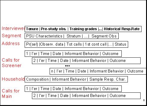
The paradata for NSFG consist of observations made by listers of sample addresses when they visit segments for the first time, observations by interviewers upon first visit and each contact with the household, call record data that accumulate over the course of the data collection, and screener data about household composition.
These data can be informative about nonresponse bias in key indicators from NSFG to the extent that they are correlated to both response propensities and key survey variables. The structure of the paradata thus resembles the nested form of the data records below:

Thus, we have data on
(a) interviewers,
(b) on the sampled segments (including segment observations by listers & interviewers), (c) on the selected address,
(d) on the date and time of visits (“calls”) for screeners and main interviews, and
(e) on the household.
These data include comments or remarks made by screener informants and by persons selected to be interviewed.
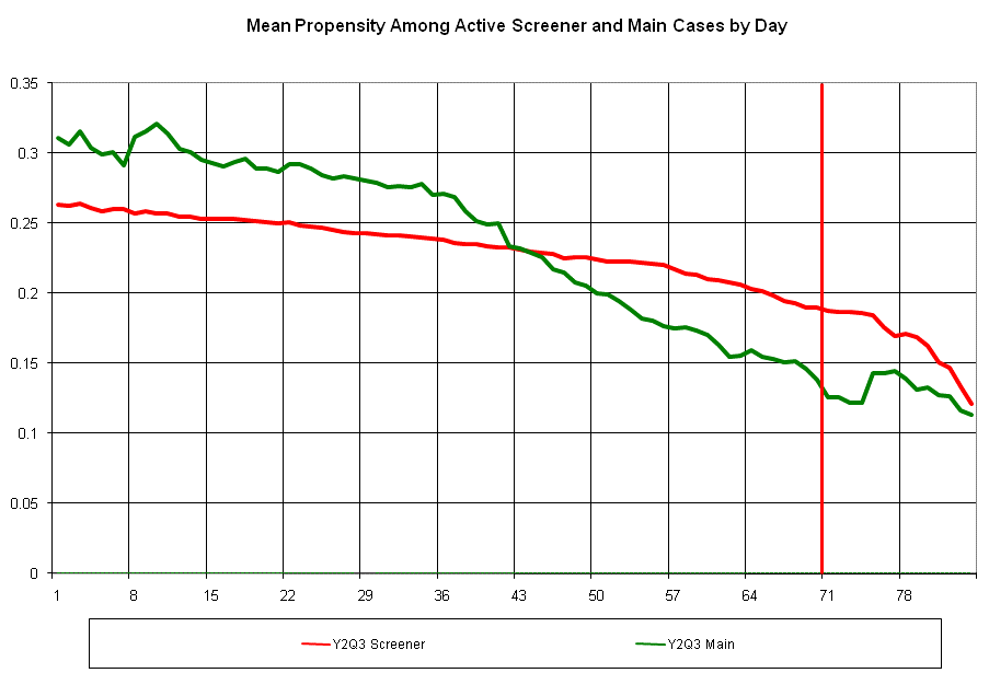
From these data we build daily discrete hazard conditional propensity models. These models estimate the likelihood for each active screener and main case that the next call will generate a successful interview. We monitor the mean probability of this event over the course of the 10-week phase 1 data collection period. These data allow us to diagnose whether more or less relative attention should be paid by interviewers to the screener interviewing versus the main interviewing, in order to achieve desirable balance in the respondent data set. The specification of these propensity models is similar to that describe in the Cycle 6 Series 1 report (Groves et al, 2005).
We track the mean probability of an active case responding daily throughout the data collection period, using graphs like that below. The graph shows a gradual decline in the likelihood of completing an interview as the data collection period proceeds, reflecting the fact that easily accessible and highly interested persons are interviewed most easily and quickly.

Sensitivity of Key Estimates to Calling Effort
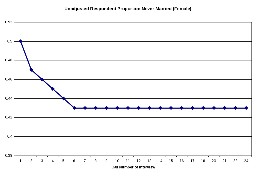
We estimate daily (unadjusted) respondent-based estimates of key NSFG variables. We plot these estimates as a function of the call number on which the interview was conducted, yielding graphs like that below.
For example, the chart below provides the unadjusted respondent estimate of the proportion of females never married, which stabilizes within the first 7 calls. That is, the combined impact of the number of interviews brought into the data set after 7 calls and the characteristics of those cases on the “ever married” variable produces no change in the unadjusted respondent estimate. For this specific measure, therefore, further calls with the phase 1 protocol have little effect.
Monitoring several of these indicators allows us guidance on minimum levels of effort that are required to yield stable results within the first phase of data collection.

Daily Monitoring of Response Rates for Main Interviews Across 12 Socio-Demographic Groups
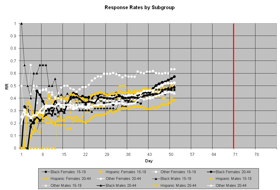
We compute response rates of main interviews (conditional on obtaining a screener interview) daily for 12 socio-demographic subgroups that are domains of the sample design and important subclasses in much of family demography (i.e., 12 age by gender by race/ethnicity groups). We estimate the coefficient of variation of these response rates daily, in an attempt to reduce that as much as possible. When the response rates are constant across these subgroups, then we have controlled one source of nonresponse bias on many NSFG national full population estimates (that bias due to true differences across the subgroups).

Randomized Responsive Design Interventions on Key Auxiliary Variables During Data Collection
We have conducted a variety of interventions on paradata that appear to indicate imbalances in the current respondent pool on key auxiliary variables. These include attempted repairs on low response rates for Hispanic male adults (20-44, based on screener data), for those households judged not to have children under 15 years of age (based on interviewer judgments upon initial visits to the housing unit), and for cases with large selection weights (based on sample selection data).
Starting in the second year of the continuous NSFG, we have made the decision that all of these interventions will be randomized to a subset of the cases eligible for the interventions. This provides measurability of the effects of the intervention with traditional statistical analysis. Some of these interventions have succeeded in raising response rates for the targeted cases; others have not. We continue to refine the intervention strategies (mostly by increasing the visibility and feedback on progress for the cases sampled for the intervention). With the completion of the final data set to be distributed in 2009 we will have formal evaluations of these interventions for both response rate and movement in key NSFG statistics.
A Two-Phase Sampling Scheme, Selecting a Probability Sample Of Nonrespondents At The End Of Week 10 Of Each Quarter
At the end of week 10 of each quarter, a probability subsample of remaining nonrespondent cases is selected. The sample is stratified by interviewer, screener/main status, selection weight, and
expected propensity to provide an interview. The second phase incentive protocol described above is offered to these cases. During year 2 analysis of the performance of the second phase
noted that outcomes for active main cases sampled into the second phase sample were better than those for screener cases; hence, the sample is disproportionately allocated to main cases (about 60% of the cases are active main interview cases). The revised incentive used in phase 2 (weeks 11 and 12 of each 12-week quarter) appears to be effective in raising the propensities of the remaining cases, bringing into the respondent pool persons who would have remained nonrespondent without the second phase.
Given the randomized nature of the second phase, we will be able to measure the impact on key NSFG statistics (as we did in Cycle 6) in an analysis to accompany the 2009 data set.
Comparison of alternative postsurvey adjustments for nonresponse
We are now examining alternative adjustment models for use with the first data set to be released in 2009. This work has pointed out to us the value in separate uses of auxiliary variables that predict likelihood of measurement and those that predict key survey variables. We have estimated correlations between some of the interviewer observations and key NSFG variables and some achieve correlations in the range of .2 to .4. These levels were found to be a minimal requirement for impact on adjustment in a multi-study evaluation of propensity model adjustments (see Kreuter et al., 2008)
References for Attachment L
Groves R, Benson G, Mosher W, et al. 2005. Plan and Operation of Cycle 6 of the National Survey of Family Growth. Vital and Health Statistics, Series 1, No. 42, August, 2005. 86 pages.
Kreuter F., Olson K., Wagner J., Yan T., Ezzati-Rice, T.M., Casas-Cordero C., Lemay
M., Peytchev A., Groves R.M., Raghunathan T.E. 2008. Using Proxy Measures and Other Correlates of Survey Outcomes to Adjust for Nonresponse: Examples from Multiple Surveys, under review at the Journal of the Royal Statistical Society.
| File Type | application/msword |
| Author | wdm1 |
| Last Modified By | Bill Mosher |
| File Modified | 2008-12-03 |
| File Created | 2008-09-25 |
© 2026 OMB.report | Privacy Policy