FINAL_HCS_SSB_ATTACH 3_STAT POWER ANALYSIS_July 2013
FINAL_HCS_SSB_ATTACH 3_STAT POWER ANALYSIS_July 2013.docx
The Healthy Communities Study: How Communities Shape Childrens Health (NHLBI)
FINAL_HCS_SSB_ATTACH 3_STAT POWER ANALYSIS_July 2013
OMB: 0925-0649
S SB
ATTACHMENT 3
HEALTHY COMMUNITIES STUDY
ASSESSMENT OF STATISTICAL POWER FOR THE
HEALTHY COMMUNITIES STUDY
1. Introduction
The NHLBI Healthy Communities Study seeks to assess the associations between characteristics of community programs and policies and childhood obesity. The number of communities included in the study design is to be chosen to be within the allocated resources available and to allow valid statistical inferences to be made about subtle associations that programs or policies (or their components) have with childhood obesity outcomes over time. The purpose of this section is to describe how study power was estimated over a variety of scenarios.
Power refers to the probability of correctly rejecting the null hypothesis that the program has zero relationship with childhood obesity when the program truly has a non-zero relationship. Effect size is the smallest non-zero association that a program can have with childhood obesity and still be considered statistically different from zero. A study design with high power will tend to reach the correct conclusion about program effectiveness more often than a design with low power. Furthermore, a study design that detects a small effect size is preferable because this design will be able to distinguish subtle levels of associations.
This document describes simulations we conducted to assess the power and effect size of the Healthy Communities Study design under a variety of scenarios. The analysis focused on two outcomes of interest: body mass index (BMI) and a binary measure of nutrition (e.g. whether the participant consumed sugar-sweetened beverages in the last seven days). A key goal of the study is to relate the outcomes of interest to a score of program/policy implementation at the community level. Section 2 describes the statistical models that we used to simulate and analyze the data. Section 3 describes the attributes that we assumed the sampled communities would have, including distributional assumptions about the program/policy score. Section 4 describes the age and gender makeup of the study participants in each sampled community. We describe how we generated the BMI data and nutrition data in Sections 5 and 6, respectively. The results of our analysis are provided in Section 7.
2. Statistical Models
We considered several statistical models for each response. For BMI, we considered a longitudinal model that had the following form
 (1)
(1)
where
 is
the lth BMI measurement from child k
attending school j in community i;
 is
the age at the time of the BMI measurement;
 is
a polynomial in the child’s age and represents the raw BMI
assuming no community program is implemented;
 is
the program/policy score at time l in community i;
 is
a random community effect (independent of program/policy score);
 is
a random school effect independent of the community;
 is
a random child effect independent of the school and the community;
and
 is
a random error independent of child, school, and community. The
random effects were drawn from a normal distribution with mean zero
and standard deviations of 0.05 for the community effect (
 ),
0.05 for the school effect (
 ),
0.19 for the child effect (
 ),
and 0.019 for the random error (
 ,
with these values established based on prior analyses of longitudinal
BMI data.
We considered a cross-sectional BMI model as well. The cross-sectional data were generated using the following equation:
 (2)
(2)
where
each term has the same meaning as Equation (1) except that the time
subscript, l, is removed. With the time effect removed, the
terms
 and
and
 both represent a random error. The model used to fit the
cross-sectional data was therefore
 (3)
(3)
with
 representing a random error whose variance is the sum of the variance
for
 and
and
 .
.
For the binary nutrition outcome, we assumed a cross-sectional model that had the following form:
 (4)
(4)
where
 is
probability that the binary outcome is present for child k
attending school j in community i;
 is
the program/policy score for community i;
 is
a random community effect (independent of program/policy score); and
 is
a random school effect independent of the community. The random
community and school effects were drawn independently from a normal
distribution with mean zero and a standard deviation of 0.05,
matching the value for the BMI models.
For
all statistical models and both outcomes, the hypothesis under
investigation is whether
 equals zero. Effect size is the smallest value of
 that provides a specified power.
3. Modeling Community Attributes
The central hypothesis under investigation explores the association between community programs or policies (and how they or their component pieces evolve over time) and BMI or PA/nutrition outcomes measured on participant children from within those communities. However, different communities could be implementing programs or policies at different levels of intensity at the time the study is conducted. Based on the study research plan, we assumed that program/policy scores would be measured on a scale between 0 and 1, where 0 means that the program is not implemented at all and 1 means that the program is implemented completely at full intensity.
Since some of the statistical models are longitudinal, we needed to develop a model that explains the change in program/policy score over time. Our simulations allowed for the program/policy scores to increase or decrease over time. The following logistic equation was used to simulate how community program/policy intensity scores changes over time:

where
 is
the program/policy score and
 is
time in years. The value of c was randomly selected from a
normal distribution with a mean of zero and a standard deviation of
1.25. This distribution allows different simulated communities to
increase or decrease program/policy scores over time at different
rates. The sign of the intercept ensures that two program/policy
score curves with equal but opposite slopes will reach 0 (for the
decreasing program/policy) or 1 (for the increasing program/policy)
after the same number of years.
Each community’s position on the program/policy score curve at the time of the baseline measurement was randomly selected from a beta distribution. The beta family of distributions places a probability on continuous values between 0 and 1. The exact shape of a particular beta distribution is determined by a combination of two parameters, and many different forms are possible that assign more weight to portions of the interval [0, 1]. For purposes of this analysis, we considered two different beta distributions: beta(1, 1), and beta(0.5, 2). A beta(1, 1) distribution is equivalent to a uniform distribution that assigns probability equally over the interval [0, 1]. It has a mean of 0.5 and a standard deviation of 0.29. A beta(0.5, 2) distribution is even more heavily weighted towards values in the low end of the interval. It has a mean of 0.33 and a standard deviation of 0.24. Figure 1 depicts the shapes of the two beta distributions used in the analysis.
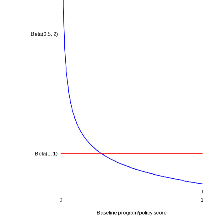
Figure 1. Distributions of Baseline Program Intensity
Figures 2a and 2b illustrate different program/policy score timelines using the two different beta distributions described above. Each figure shows 15 randomly sampled curves, and each of the 15 curves has a different slope and a different initial score. The timeline in each figure starts ten years before the baseline year and ends at the baseline year. Figure 2a indicates a roughly uniform pattern to the program/policy scores at the baseline year, as would be expected when the intitial score is sampled from a beta(1, 1) distribution. In Figure 2b, most of the program/policy scores at the baseline year are near zero, as would be expected when the intial score is sampled from a beta distribution that is skewed to the right. In both plots, most of the lines have a relatively gradual slope. Furthermore, roughly half of the lines have a positive slope and the other half have a negative slope. These features are to be expected since the slopes were drawn from a normal distribution that is centered at zero.
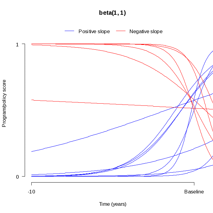
Figure 2a. Sampled Program Timelines Using Beta(1, 1) Distribution for Initial Intensity
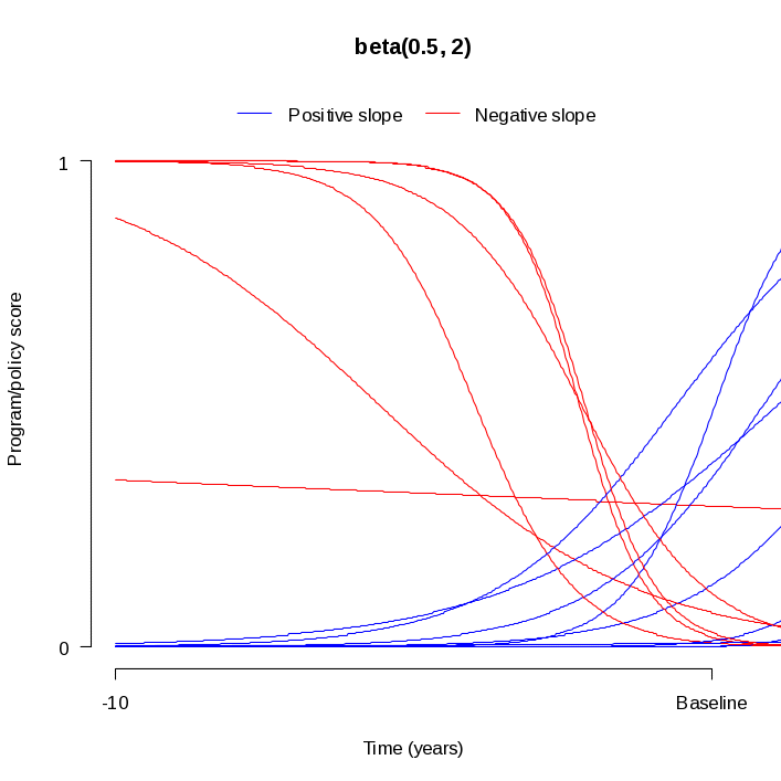
Figure 2b Sampled Program Timelines Using Beta(0.5, 2) Distribution for Initial Intensity
Once a community’s baseline score was simulated, we determined a baseline time on the score growth curve for that community. This time was used to determine the relative timing of the BMI measurements before baseline obtained from the medical record abstraction. The relative times were then used to find the community’s intensity level at the time when the retrospective BMI measurements were taken.
Figure 3 illustrates this concept using BMI measurements from a child in a community with an increasing program/policy score curve. The baseline score is sampled first, and the curve is used to determine a baseline time that represents how far along the community has progressed in implementing the program/policy. This time is denoted by b in Figure 3. We then calculated the timing of measurement recordings relative to the baseline time using the parameters of the study design and a random process for the timing of medical visits (described in more detail in Section 4). These times were then input into the growth curve formulas to obtain a program/policy intensity score level at the time the measurement was taken. For example, suppose the child represented by Figure 3 was found to have a medical visit 2.1 years before baseline. The value on the growth curve at time (b – 2.1) years would be used to estimate the program/policy intensity score level at the time of the medical visit.
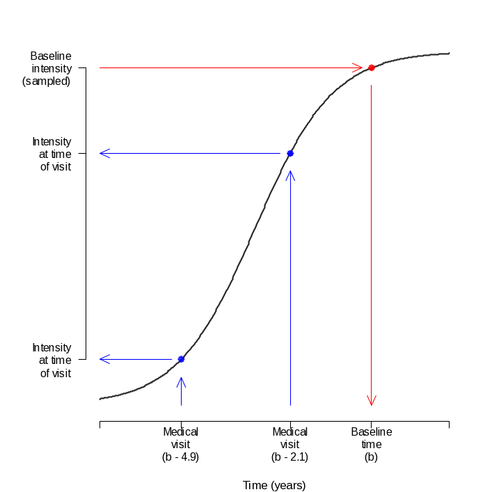
Figure 3. Illustration of Using Growth Curves to Estimate Program/Policy Score Levels
4. Sampling of Participant Gender and Ages
We conducted power calculations for a design with 264 communities and 9 participants per grades K-8 from each community, yielding a total of 21,384 participants. For the simulation, patterned data were generated for each community that matches the required number of children at each grade level. Every other grade had 4 males and 5 females, with the grades in between having 5 males and 4 females. In one-half of the communities, this pattern started with 4 males and 5 females in the kindergarten class, with the pattern reversed for the other half of the communities. We assumed participants in grades K-5 would be recruited from an elementary school and participants in grades 6-8 would be recruited from a middle school.
For each community, we simulated the number of elementary and middle schools that would agree to participate in the study. We assumed two elementary schools from the same community would agree to participate with a probability of 80%; otherwise, only one elementary school would agree to participate. Similarly, we assumed two middle schools from the same community would agree to participate with a probability of 65%; otherwise, only one middle school would agree to participate. In simulations where two elementary and/or middle schools were recruited from a community, participants were randomly assigned to a school with a probability if 50%. When only one elementary and/or middle school was recruited, we assumed all participants from a grade range came from the same school.
The exact age of each child at the time of the in-person measurement was sampled from a range of ages that corresponds to each grade. We assumed that September 1 was the start of the school year, June 1 was the end of the school year, and a December 1 was the birthday cutoff for each grade. Thus, the youngest child in the class on September 1 would be the grade plus 4.75, and the oldest child in the class on that day would be the grade plus 5.75 (e.g., 5.75 to 6.75 for first grade, 6.75 to 7.75 for second grade). As the visit date to the community varies from September 1 to June 1, so does the range of ages. On June 1, the youngest child in the class would be the grade plus 5.5 and the oldest child would be the grade plus 6.5 (e.g., 6.5 to 7.5 for first grade, 7.5 to 8.5 for second grade). Assuming a uniform distribution of visit dates between September 1 and June 1, and assuming a uniform distribution of ages between the range of possible ages for a given visit date, the distribution of ages in a particular grade follow a triangle distribution with a minimum of (grade + 4.75), a maximum of (grade + 6.5), and a mode of (grade + 5.625). Our simulations used this triangle distribution to sample ages for each grade.
Since there are no follow-up visits planned for the current design, the timing of the community visits was not accounted for in the simulations.
5. Constructing BMI Data
The simulations assumed that a BMI measurement would be obtained from each child during the in-person assessment. Furthermore, retrospective BMI measurements would be available from medical records for 70% of the participants.
The medical record abstraction data from Wave 1 yielded retrospective BMI trajectories for 65 different participants. We examined the 65 BMI trajectories to get an understanding of the number of BMI measurements per participant, the spacing between measurements, the timing of the earliest BMI measurement, and the timing of the most recent BMI measurement. Table 1 provides summary statistics for these values across all participants regardless of age; it is these summary statistics that are used to inform our power studies. The summary statistics were calculated across all ages because we did not find any statistically significant differences in these values for different ages.
Table 1. Summary Statistics for the Timing of BMI Measurements
|
n |
Mean |
Std Dev |
Min |
Max |
Number of BMI measurements |
65 |
5.66 |
5.00 |
1.00 |
23.00 |
Average spacing between BMI measurements |
51 |
1.19 |
1.18 |
0.08 |
6.08 |
Years since earliest BMI measurement |
65 |
6.07 |
3.95 |
0.47 |
15.01 |
Years since most recent BMI measurement |
65 |
1.97 |
2.11 |
-0.14 |
8.82 |
The summary statistics in the above table were used to parameterize general beta distributions from which we sampled the four timing aspects of the BMI measurements. The shapes of the four distributions are depicted in Figure 4.
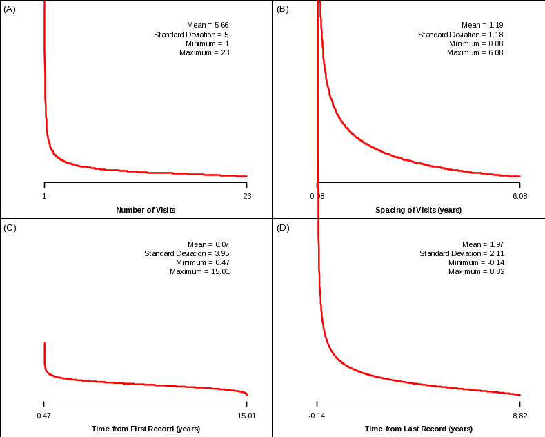
Figure 4. Distributions Used to Simulate Timing of BMI Measurements: (A) Number of visits where both height and weight were measured; (B) Number of years between visits; (C) Number of years since earliest BMI record; (D) Number of years since most recent BMI record
Once a set of values for the four timing aspects is sampled, we combined them to form a simulated sequence of ages at which a BMI measurement is obtained from the medical records. The average of these sequences over all of the simulated participants will match the summary statistics from the Wave 1 data, but individual sequences will vary due to randomness in the simulation.
The simulated medical history along with the age at the time of the HCS in-home visit provided a sequence of ages at which the subject’s BMI was measured. We used these ages, and the child’s gender to determine a raw BMI from CDC’s 2000 BMI-for-age percentiles (http://www.cdc.gov/growthcharts/html_charts/bmiagerev.htm). The raw BMI is the BMI that the child would have if there were no community programs implemented.
Each
child’s measured BMI was simulated using the statistical models
in Section 2. In that model,
 represents the raw BMI following the median BMI in the CDC tables.
The community’s program/policy score,
 ,
was determined from the intensity growth curves (illustrated in
Figure 3). The random child effect (
 )
captures any child-specific deviation from the median BMI in the CDC
tables.
6. Constructing Binary Outcomes
Our
simulation of binary outcomes was more straightforward than our
simulation of BMI measurements since the former does not rely on a
history of medical visits. Each child was assumed to complete a
dietary assessment during the in-home visit. The binary outcome
based on that assessment was sampled from a Bernoulli distribution.
The probability of a success was determined by the statistical model
described in Section 2. The community’s program/policy score,
 ,
was determined from the sampled score at baseline.
The
value of
 was calculated such that the prevalence of the outcome was equal to
0.5. The prevalence is equal to the unconditional probability of the
outcome and involves integrating over the distribution of the
 values. Since two different beta distributions were used for the
program/policy score, the simulation used two different values of
 :
-0.475 for the beta(1, 1) distribution and -0.189 for the beta(0.5,
2) distribution.
7. Results
Using
the methods described above, we replicated study data 500 times for
each baseline intensity distribution depicted in Figure 1. For each
replication, we fit the appropriate statistical model to the
simulated data. We recorded the point estimate of
 for each model fit. Taking the standard deviation of the 500 point
estimates of
 provided us with an estimate of the true standard error of
 .
.
Using
our estimate of the standard error of
 ,
we can calculate the combinations of power and effect size attainable
from the study design. For a two-sided test, the effect size is
determined from the following equation:

where
 is
the standard error estimated from the simulation,
 is
the power,
 is
the significance level of the test, and
 is
the 100*uth percentile from a standard
normal distribution.
After the data are collected, a researcher may be interested in assessing the relationships between a program and BMI in a particular age group. There are at least two possible ways of doing this type of analysis for a longitudinal model. One approach would use all data that were measured when a subject’s age was within the age group of interest regardless of the subject’s age at the in-person assessment, allowing analyses of how community programs/policies (and how they change over time) influence child obesity outcomes within specific age groups. For example, suppose a subject who was 15 years old at the in-person assessment was found to have medical records containing BMI information when she was 4 years old. Those records could be included in an analysis focusing on the 3-4 year-old age group. A second approach would use all data ever measured on an individual whose in-person age fell within the age group of interest, enabling specific cohort analyses. For example, a study focusing on 3-4 year-olds would include all data collected on those children that were ages 3 or 4 at the in-person assessment. Our simulation study addressed both of these research approaches.
Our power calculation results are presented in terms of the percent change in effect size detectable for a unit change in program/policy score. The calculated effect sizes assume 80% power for conducting a two-sided test of significance at α = 0.05. For the BMI models, the percent change in effect size is the smallest percentage difference in BMI between a community with score 0 and a community with score 1 that would be considered statistically significant at α = 0.05 and 80% power. For the binary model, the percent change in effect size is the smallest percentage point difference in the proportion of children with the outcome between a community with score 0 and a community with score 1 that would be considered statistically significant at α = 0.05 and 80% power.
| File Type | application/vnd.openxmlformats-officedocument.wordprocessingml.document |
| Author | Chris Sroka |
| File Modified | 0000-00-00 |
| File Created | 2021-01-29 |
© 2026 OMB.report | Privacy Policy