Attachment X - Data Analysisor Change in Diary Placement
Attachment X - Diary Placement Day and Expenditure Cycles - April 2015.docx
Consumer Expenditure Surveys: Quarterly Interview and Diary
Attachment X - Data Analysisor Change in Diary Placement
OMB: 1220-0050
The Placement Date’s Effect
on Monthly Expenditure Cycles
in the Diary Survey
April, 2015
Introduction
CE’s diaries are placed with respondents uniformly throughout the month to make sure the expenditures reported on them accurately reflect all of the expenditures made by respondents, including items with monthly expenditure cycles. For example, the rent of an apartment is usually paid on the first day of the month, so placing diaries uniformly throughout the month ensures that one-fourth of the weekly diaries have a rental expenditure reported on them just like renters make their payments in one-fourth of the weeks of a month. This self-weighting feature of the survey is crucial to producing unbiased expenditure estimates.
Some UCCs have stronger monthly expenditure cycles than others. Rent has a strong monthly cycle, but milk and bananas have weak or nonexistent cycles because they are purchased throughout the month. Since many of the UCCs with strong monthly expenditure cycles are taken from the Interview survey in the integration process and not from the Diary survey, some people have wondered whether placing diaries uniformly throughout the month is really that crucial. This memo examines that question.
The data analysis presented here shows that when the universe of UCCs is limited to those in the Diary survey used in the integration process, the monthly expenditure cycles are considerably weaker and may not even exist. At the national level the expenditure cycles observed in the “All Items” category and nine major groups were all below the statistically significant level. When the data were partitioned into a large number of small subsets 5% of them had expenditure cycles that were statistically significant at the .05 level, and 1% of them had expenditure cycles that were significant at the .01 level, which is consistent with a null hypothesis of cycles not existing. Both of these observations suggest the few cycles observed in the data may have been the result of normal random fluctuations expected in the survey’s data and not from any true underlying expenditure cycles.
Two Kinds of Placement Days
Before examining the effect of a diary’s placement strategy, it is important to know there are two kinds of placement days – the earliest placement day and the actual placement day. When CE’s field representatives are given their work assignments every address has a 7-day window in which a diary must be placed at a household. The first day of the 7-day window is the earliest placement day, and the day on which the diary is actually placed is the actual placement day.
The earliest placement days are uniformly distributed throughout the year. The Census Bureau does it by dividing its yearly sample of addresses into 365 equal parts with each part getting a different earliest placement day.1 The purpose is to make sure expenditures from every day of the year are fully represented in the survey, including parts of the year with seasonal expenditures like turkeys in November and college tuition in September, and parts of the month with cyclical expenditures like rent and utilities.
Here are graphs showing the monthly cycle of expenditures by earliest and actual placement days. The data are from 2009-2013, and the average annual expenditures are computed by multiplying the weekly expenditures by 52.
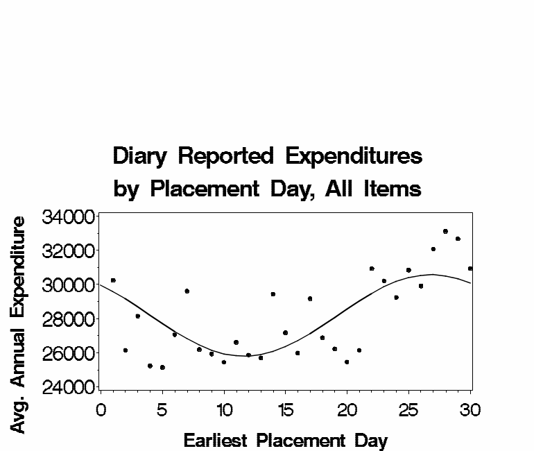
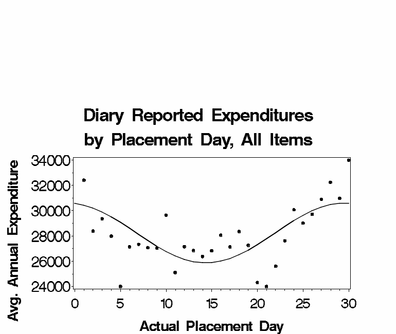
Several things can be observed in these graphs, but the most important thing to observe is the existence of cycles. The average annual reported expenditure ranges from $26,000 to $31,000 depending on the part of the month in which the diaries are placed. If all diaries were placed at the beginning or end of the month CE’s expenditure estimates would be too high ($31,000), and if all diaries were placed in the middle of the month CE’s expenditure estimates would be too low ($26,000). These cycles are the reason diaries are placed uniformly throughout the month – to make sure the peaks and troughs of the expenditure cycle are reflected in the data as well as everything in between. The graphs also show the earliest placement day precedes the actual placement day by three days, but again the existence of cycles is the most important thing to observe.
Measuring the Strength of Monthly Expenditure Cycles
As mentioned above, some UCCs have stronger monthly expenditure cycles than others. There are many ways the strength of monthly cycles can be measured, but in this memo they are measured by fitting a cosine function to the data and then measuring the percent of the data’s variance it explains. This statistic is called “R-squared.” It is a number between 0 and 1, and higher values indicate stronger monthly cycles.
To be precise, here is the cosine function used in this memo to model a UCC’s expenditures throughout the month: 2

where: |
|
|
xt |
= |
The average annualized expenditure among all CUs whose diary was placed on the t-th day of the month (t = 1,2,…,31) |
0 |
= |
The average annualized expenditure on the UCC across all 31 placement days |
1 |
= |
The maximum expected deviation from the average annualized expenditure over all 31 placement days (the amplitude) |
2 |
= |
The day of the month with peak expenditures (the phase shift) |
t |
= |
The error term. This is the difference between the observed values and the modeled values. |
This is a cyclical model of expenditures with a period of 30.4 days. Except for the period, the rest of the model’s parameters are estimated from the data using the method of least squares. The model focuses on a diary’s placement day rather than a respondent’s expenditure day because we have control over the placement day. Then this is the R-squared statistic used to measure the strength of the monthly cycles:

The numerator is the variance of the data assuming expenditures follow a cosine function; the denominator is the variance of the data assuming expenditures are constant throughout the month; and one minus the ratio is the percent of variance explained by the cosine function.
UCCs with the Strongest Monthly Expenditure Cycles
Based on the R-squared statistic, these are the UCCs with the strongest monthly expenditure cycles:
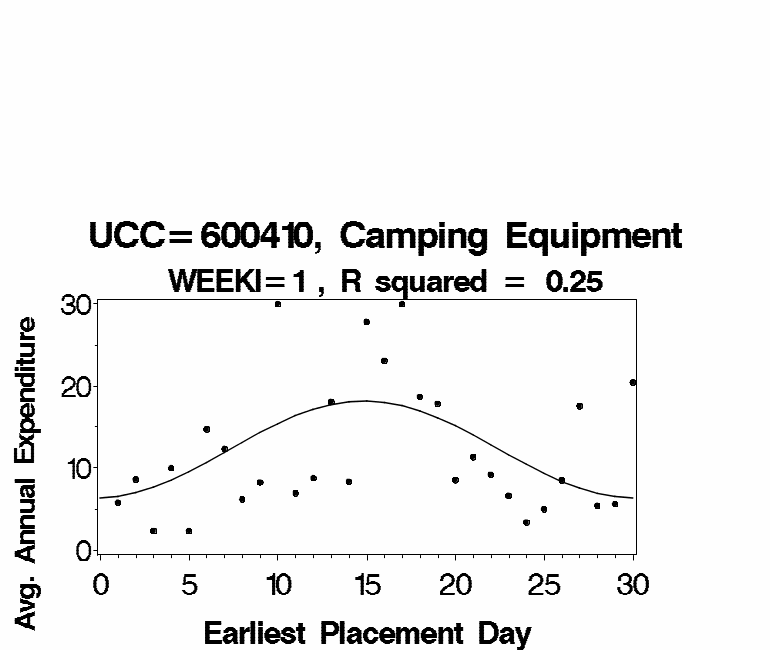
Top 20 UCCs with the Strongest Monthly Expenditure Cycles (Highest R-Squared Statistics)
|
||||||||
|
|
Earliest Placement Day |
Actual Placement Day |
|||||
UCC |
Source |
WEEKI=1 |
WEEKI=2 |
WEEKI=1+2 |
WEEKI=1 |
WEEKI=2 |
WEEKI=1+2 |
|
1. 210110 Rent |
I |
0.88 |
0.81 |
0.86 |
0.81 |
0.79 |
0.87 |
|
2. 009000 Mortgage Payment |
--- |
0.73 |
0.64 |
0.74 |
0.64 |
0.67 |
0.77 |
|
3. 580000 Health Insurance not specified |
--- |
0.51 |
0.33 |
0.49 |
0.38 |
0.04 |
0.40 |
|
4. 004190 Gifts not specified |
--- |
0.40 |
0.07 |
0.05 |
0.17 |
0.03 |
0.02 |
|
5. 060310 Other Poultry |
D |
0.37 |
0.38 |
0.48 |
0.22 |
0.07 |
0.17 |
|
6. 270210 Water/Sewer Maintenance |
I |
0.37 |
0.52 |
0.45 |
0.31 |
0.40 |
0.53 |
|
7. 230900 Property Management |
I |
0.36 |
0.21 |
0.19 |
0.46 |
0.30 |
0.57 |
|
8. 520531 Parking Fees in Home City |
I |
0.36 |
0.22 |
0.28 |
0.19 |
0.16 |
0.25 |
|
9. 270410 Garbage/Trash Collection |
I |
0.34 |
0.25 |
0.32 |
0.53 |
0.05 |
0.38 |
|
10. 270310 Cable/Satellite Television Services |
I |
0.33 |
0.11 |
0.41 |
0.31 |
0.06 |
0.28 |
|
11. 260110 Electricity |
I |
0.33 |
0.49 |
0.28 |
0.30 |
0.30 |
0.48 |
|
12. 030210 Chuck Roast |
D |
0.33 |
0.01 |
0.16 |
0.23 |
0.02 |
0.08 |
|
13. 610901 Fireworks |
D |
0.31 |
0.19 |
0.24 |
0.25 |
0.06 |
0.24 |
|
14. 550330 Supp./Conv. Medical Equipment |
I |
0.27 |
0.02 |
0.13 |
0.29 |
0.05 |
0.06 |
|
15. 340610 Repair of TV/Radio/Sound Equip. |
I |
0.26 |
0.11 |
0.17 |
0.10 |
0.02 |
0.11 |
|
16. 600410 Camping Equipment |
D |
0.25 |
0.04 |
0.18 |
0.14 |
0.04 |
0.08 |
|
17. 310220 Video Cassettes, Tapes, Discs |
D |
0.25 |
0.01 |
0.14 |
0.24 |
0.06 |
0.09 |
|
18. 320904 Closet and Storage Items |
D |
0.25 |
0.12 |
0.28 |
0.26 |
0.05 |
0.26 |
|
19. 440110 Shoe Repair |
I |
0.24 |
0.05 |
0.21 |
0.17 |
0.06 |
0.06 |
|
20. 010310 Rice |
D |
0.24 |
0.01 |
0.14 |
0.11 |
0.14 |
0.24 |
|
A few things can be observed in this table. First, there are six sets of R-squared values, three for the earliest placement day and three for the actual placement day. As the bold font indicates, emphasis in this memo is placed on the strength of the relationship between an address’s earliest placement day and the expenditures reported in the first week’s diary. The earliest placement day is emphasized over the actual placement day because we have more control over the earliest placement day, and the first week’s expenditures are emphasized over the second week’s expenditures (or both weeks combined) because the Gemini project is planning on the Diary portion of the survey lasting only one week.
Second, the first two UCCs on the list (Rent and Mortgage Payments) have high R-squared values indicating strong monthly expenditure cycles, and after that the R-squared values drop off quickly. Simulations show that R-squared values over 0.30 are statistically significant, R-squared values under 0.20 are not significant, and R-squared values between 0.20 and 0.30 are borderline cases. This means the first 13 UCCs on the table have statistically significant R-squared values, and the remaining seven UCCs have borderline R-squared values. 3
Third, nine of the top ten UCCs are not taken from the Diary survey in the integration process. Six are taken from the Interview survey and three are not considered to be expenditures. Only one of the top ten UCCs (Other Poultry) is used in the integrated expenditure estimates. This means nine of the top ten UCCs are irrelevant, so their data should be removed from the “All Items” graph previously shown and the results should be re-evaluated.
Fourth, the R-squared values in different columns of the table are quite variable. For example, in “Health insurance not specified” they range from 0.04 to 0.51; in “Gifts not specified” they range from 0.02 to 0.40; and in “Other Poultry” they range from 0.07 to 0.48. The wide range of R-squared values suggest that the conclusions drawn from the data may be sensitive to the way the data are analyzed, and therefore the conclusions may not be as reliable as they first seem.
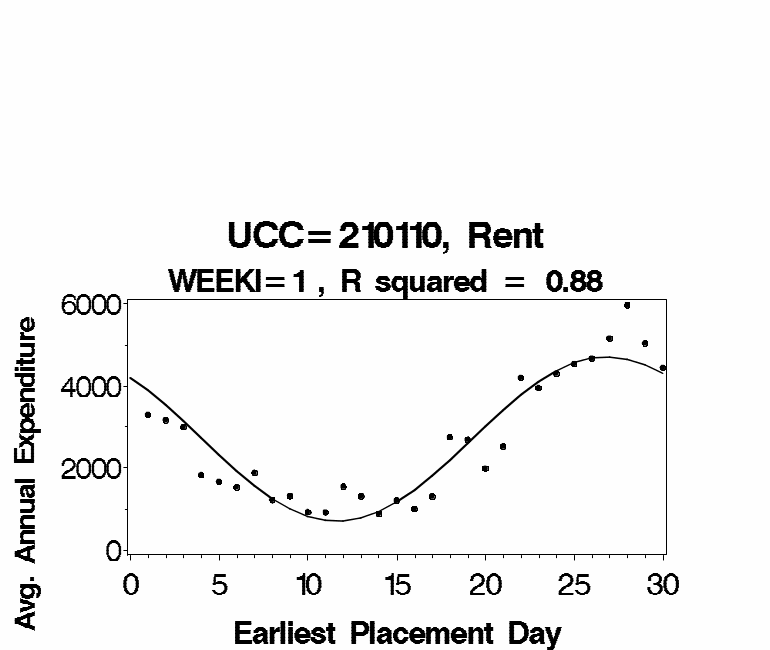
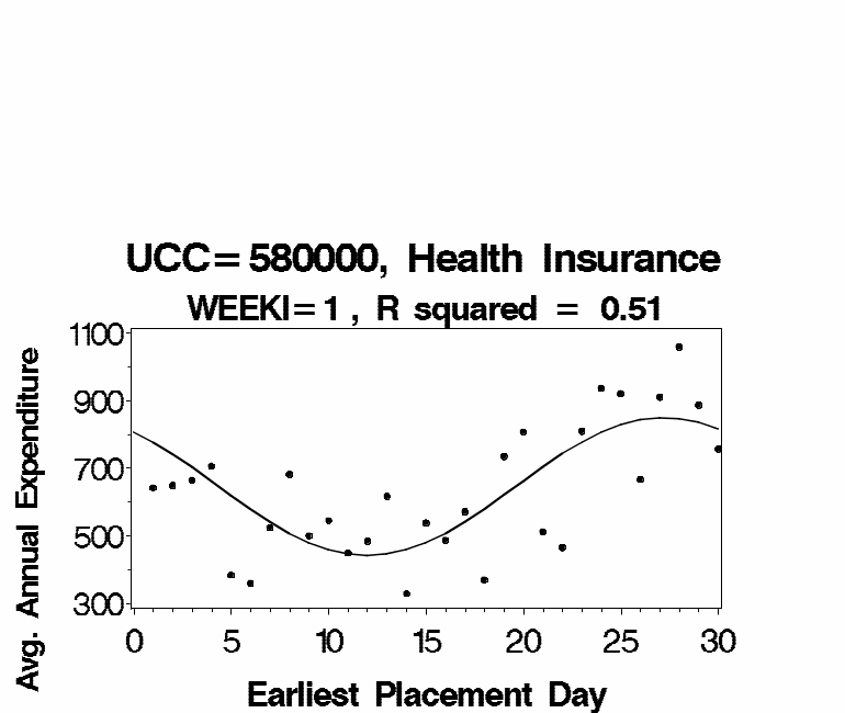
And finally, here are graphs of “Rent,” “Health Insurance not specified” and “Camping Equipment” to show what expenditure data with different R-squared values look like. Expenditures with an R-squared value of 0.88 have a strong clearly-defined cycle; expenditures with an R-squared value of 0.51 have a noticeably weaker cycle; and expenditures with an R-squared value of 0.25 have an even weaker cycle.
The Effect of Integration on the Strength of Monthly Cycles
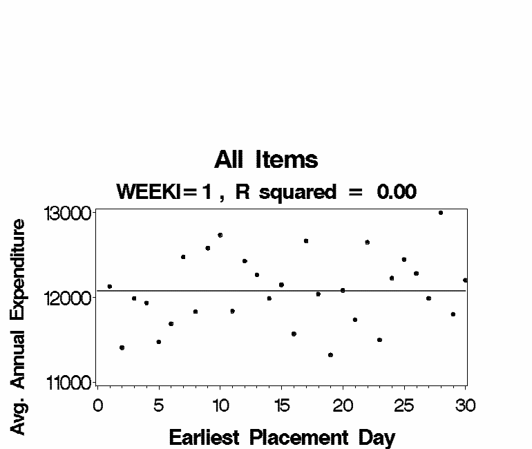
As we all know, CE consists of two surveys (Diary and Interview) with overlapping universes of UCCs, and integration is the process of deciding which survey’s data to use in the official expenditure estimates. In 2009-2013 the Diary’s expenditure databases (FDB, MLS, CLO, OTH) had 550 UCCs, and 278 of them were used in the official integrated expenditure estimates.4 By limiting the data to those 278 UCCs and summarizing them by major groups, the monthly expenditure cycles were found to be weaker than when all UCCs were used. This confirms the original hypothesis some people made before the study started about UCCs with stronger monthly cycles being taken from the Interview survey and UCCs with weaker monthly cycles being taken from the Diary survey. These weaker cycles can be seen in the table below where the R-squared values of the reduced dataset are smaller.
The Strength of Monthly Expenditure Cycles by Major Group (R-Squared Statistics)
Diary Survey, 2009-2013, WEEKI=1
|
||||
|
All UCCs in the Diary Database |
All UCCs in the Diary Database used in Integrated Expenditure Estimates |
||
Major Group |
Earliest Placement Day |
Actual Placement Day |
Earliest Placement Day |
Actual Placement Day |
1. Shelter |
0.88 |
0.80 |
--- |
--- |
2. All Items |
0.49 |
0.41 |
0.00 |
0.09 |
3. Utilities, Fuels, and Public Services |
0.32 |
0.30 |
--- |
--- |
4. Entertainment |
0.17 |
0.12 |
0.08 |
0.02 |
5. Housing – excl. shelter, utilities |
0.15 |
0.07 |
0.11 |
0.08 |
6. Other |
0.14 |
0.11 |
0.07 |
0.18 |
7. Food Away from Home |
0.07 |
0.18 |
0.07 |
0.18 |
8. Transportation – excl. gas/oil |
0.05 |
0.05 |
0.16 |
0.06 |
9. Healthcare |
0.04 |
0.05 |
0.09 |
0.09 |
10. Gasoline and Motor Oil |
0.03 |
0.08 |
--- |
--- |
11. Apparel |
0.03 |
0.07 |
0.04 |
0.07 |
12. Food at Home |
0.02 |
0.05 |
0.02 |
0.05 |
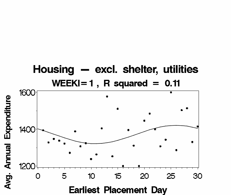
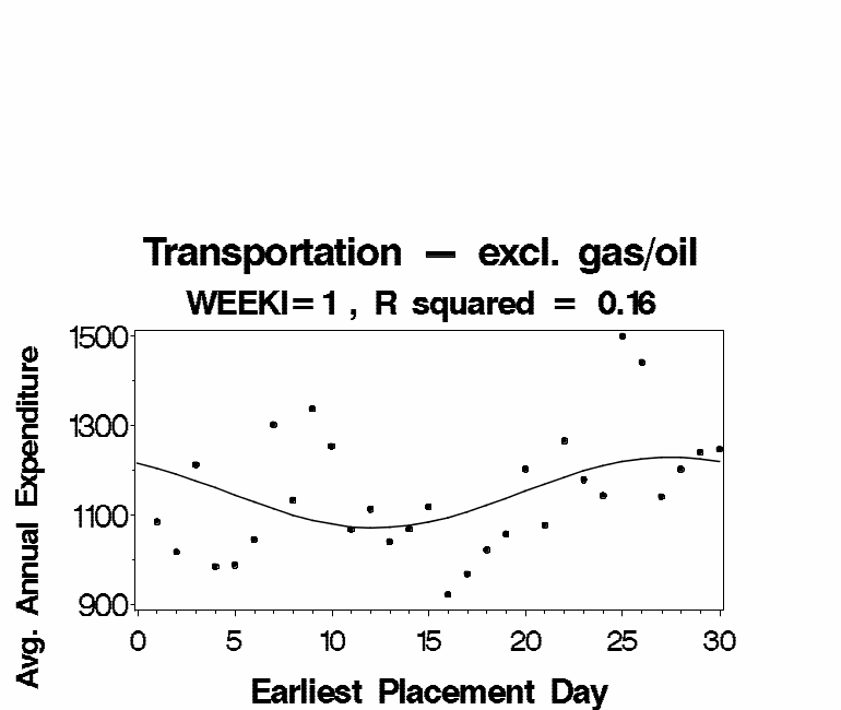
Here the R-squared value for “All Items” dropped from 0.49 to 0.00; the R-squared value for “Entertainment” dropped from 0.17 to 0.08; the R-squared value for “Housing – excl. shelter, utilities” dropped from 0.15 to 0.11; and so on. However, the big thing to notice is that the R-squared values in the reduced dataset are all below 0.20 which means they are not statistically significant, which means the resulting expenditure cycles are very weak or nonexistent. Here are graphs of “All Items” and the two major groups with the highest R-squared values showing their weak or nonexistent cycles.
The Effect of Demographic Characteristics on the Strength of Monthly Cycles
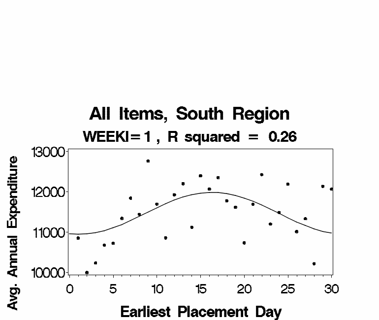
The table below shows the strength of monthly expenditure cycles for the 9 major groups having UCCs taken from the Diary survey in the integration process and 57 demographic characteristics. Check marks show the R-squared values that are statistically significant (one checkmark means the R-squared value is greater than 0.20, and two checkmarks means it is greater than 0.30). A quick glance at the table reveals two observations. First, very few R-squared statistics are statistically significant. And second, there is no clear pattern to where the statistically significant R-squared values are located. Both of these observations suggest that expenditure cycles may not exist and the few cycles observed may be the result of normal random fluctuations expected in the survey’s data.
The Strength of Monthly Expenditure Cycles in 9 Major Groups and 57 Demographic Characteristics
R-Squared Statistics for the 278 Diary UCCs used in the Integrated Expenditure Estimates
Diary Survey, 2009-2013, WEEKI=1, Earliest Placement Day = R-squared over 0.30, = R-squared over 0.20
|
|||||||||||
|
Major Group |
||||||||||
|
All Items |
Apparel |
Entertainment |
Food Away from Home |
Food at Home |
Health care |
Housing – excl. shelter, utilities |
Other |
Transportation – excl. gas/oil |
Avg |
SD |
All CUs |
.00 |
.04 |
.08 |
.07 |
.02 |
.09 |
.11 |
.07 |
.16 |
.07 |
.05 |
Age of reference person = under 30 |
.11 |
.06 |
.15 |
.05 |
.06 |
.02 |
.11 |
.01 |
.13 |
.08 |
.05 |
Age of reference person = 30-39 |
.14 |
.19 |
.02 |
.30 |
.00 |
.17 |
.05 |
.10 |
.04 |
.11 |
.10 |
Age of reference person = 40-49 |
.01 |
.02 |
.09 |
.02 |
.02 |
.02 |
.03 |
.01 |
.00 |
.02 |
.03 |
Age of reference person = 50-59 |
.01 |
.02 |
.15 |
.01 |
.12 |
.04 |
.14 |
.03 |
.07 |
.06 |
.06 |
Age of reference person = 60-69 |
.01 |
.02 |
.07 |
.10 |
.17 |
.11 |
.18 |
.01 |
.17 |
.09 |
.07 |
Age of reference person = 70+ |
.07 |
.16 |
.03 |
.00 |
.02 |
.14 |
.04 |
.04 |
.00 |
.06 |
.06 |
CU Tenure = Owner with mortgage |
.00 |
.16 |
.17 |
.01 |
.07 |
.03 |
.21 |
.00 |
.10 |
.08 |
.08 |
CU Tenure = Owner without mortgage |
.03 |
.06 |
.24 |
.14 |
.10 |
.24 |
.01 |
.08 |
.06 |
.11 |
.09 |
CU Tenure = Owner unknown mortgage status |
.17 |
.03 |
.11 |
.09 |
.12 |
.16 |
.10 |
.09 |
.15 |
.11 |
.04 |
CU Tenure = Renter |
.01 |
.02 |
.02 |
.05 |
.26 |
.03 |
.00 |
.02 |
.02 |
.05 |
.08 |
CU Tenure = Other |
.09 |
.07 |
.19 |
.03 |
.03 |
.00 |
.05 |
.04 |
.01 |
.06 |
.06 |
Education of reference person = Less than HS |
.04 |
.06 |
.02 |
.06 |
.17 |
.03 |
.04 |
.03 |
.02 |
.05 |
.05 |
Education of reference person = HS graduate |
.12 |
.29 |
.07 |
.31 |
.03 |
.20 |
.03 |
.01 |
.02 |
.12 |
.12 |
Education of reference person = Some college, no degree |
.05 |
.10 |
.01 |
.07 |
.04 |
.07 |
.00 |
.10 |
.00 |
.05 |
.04 |
Education of reference person = AA degree |
.01 |
.03 |
.04 |
.09 |
.11 |
.01 |
.04 |
.08 |
.04 |
.05 |
.04 |
Education of reference person = BA,BS degree |
.00 |
.04 |
.11 |
.02 |
.04 |
.06 |
.03 |
.06 |
.13 |
.05 |
.04 |
Education of reference person = Beyond BA,BS |
.05 |
.09 |
.02 |
.00 |
.01 |
.06 |
.21 |
.02 |
.22 |
.07 |
.08 |
Family type = Married couple only |
.01 |
.09 |
.08 |
.05 |
.02 |
.07 |
.02 |
.02 |
.02 |
.04 |
.03 |
Family type = Married couple, own children only, oldest child<6 |
.02 |
.11 |
.11 |
.01 |
.03 |
.07 |
.01 |
.17 |
.05 |
.07 |
.06 |
Family type = Married couple, own children only, Oldest child>=6, <=17 |
.00 |
.15 |
.02 |
.13 |
.01 |
.00 |
.04 |
.03 |
.10 |
.05 |
.06 |
Family type = Married couple, own children only, oldest child>17 |
.06 |
.04 |
.27 |
.07 |
.02 |
.17 |
.00 |
.05 |
.11 |
.09 |
.09 |
Family type = All other married couple families5 |
.13 |
.08 |
.04 |
.14 |
.14 |
.04 |
.04 |
.15 |
.07 |
.09 |
.05 |
Family type = One parent, male, own children, at least one age <18 |
.08 |
.05 |
.13 |
.02 |
.02 |
.10 |
.20 |
.02 |
.12 |
.08 |
.06 |
Family type = One parent, female, own children, at least one age <18 |
.15 |
.11 |
.03 |
.01 |
.15 |
.01 |
.01 |
.03 |
.04 |
.06 |
.06 |
Family type = Single |
.05 |
.06 |
.00 |
.07 |
.06 |
.03 |
.17 |
.03 |
.22 |
.08 |
.07 |
Family type = Other |
.01 |
.01 |
.00 |
.20 |
.02 |
.02 |
.09 |
.06 |
.09 |
.06 |
.06 |
Before-tax income = <=$0 |
.03 |
.09 |
.02 |
.13 |
.01 |
.16 |
.05 |
.01 |
.08 |
.07 |
.06 |
Before-tax income = $1-$10,000 |
.05 |
.07 |
.08 |
.02 |
.00 |
.10 |
.11 |
.01 |
.14 |
.06 |
.05 |
Before-tax income = $10,001-$20,000 |
.21 |
.07 |
.00 |
.07 |
.17 |
.06 |
.16 |
.01 |
.04 |
.09 |
.07 |
Before-tax income = $20,001-$30,000 |
.02 |
.09 |
.05 |
.22 |
.05 |
.19 |
.01 |
.14 |
.03 |
.09 |
.08 |
Before-tax income = $30,001-$40,000 |
.02 |
.12 |
.03 |
.06 |
.15 |
.02 |
.03 |
.04 |
.05 |
.06 |
.05 |
Before-tax income = $40,001-$50,000 |
.04 |
.04 |
.02 |
.11 |
.06 |
.08 |
.06 |
.02 |
.05 |
.05 |
.03 |
Before-tax income = $50,001-$60,000 |
.02 |
.11 |
.01 |
.05 |
.18 |
.10 |
.04 |
.04 |
.00 |
.06 |
.06 |
Before-tax income = $60,001-$70,000 |
.07 |
.01 |
.03 |
.01 |
.01 |
.07 |
.02 |
.01 |
.06 |
.03 |
.03 |
Before-tax income = $70,001-$80,000 |
.05 |
.14 |
.14 |
.16 |
.07 |
.01 |
.25 |
.05 |
.03 |
.10 |
.08 |
Before-tax income = $80,001-$90,000 |
.01 |
.08 |
.01 |
.03 |
.00 |
.11 |
.00 |
.07 |
.10 |
.05 |
.04 |
Before-tax income = $90,001-$100,000 |
.03 |
.00 |
.01 |
.07 |
.10 |
.02 |
.06 |
.10 |
.00 |
.04 |
.04 |
Before-tax income = $100,001-$120,000 |
.17 |
.04 |
.29 |
.03 |
.01 |
.07 |
.16 |
.05 |
.26 |
.12 |
.10 |
Before-tax income = $120,001-$140,000 |
.05 |
.01 |
.03 |
.00 |
.14 |
.07 |
.04 |
.01 |
.01 |
.04 |
.04 |
Before-tax income = $140,001-$160,000 |
.01 |
.04 |
.12 |
.11 |
.02 |
.13 |
.04 |
.01 |
.00 |
.05 |
.05 |
Before-tax income = $160,001-$180,000 |
.05 |
.03 |
.03 |
.15 |
.03 |
.02 |
.03 |
.11 |
.03 |
.05 |
.05 |
Before-tax income = $180,001-$200,000 |
.04 |
.08 |
.07 |
.16 |
.13 |
.00 |
.21 |
.00 |
.05 |
.08 |
.07 |
Before-tax income = >$200,000 |
.01 |
.06 |
.07 |
.02 |
.04 |
.08 |
.03 |
.06 |
.11 |
.05 |
.03 |
PSU size class = A PSUs |
.01 |
.00 |
.01 |
.04 |
.09 |
.00 |
.20 |
.06 |
.14 |
.06 |
.07 |
PSU size class = X PSUs |
.00 |
.11 |
.09 |
.02 |
.02 |
.00 |
.00 |
.11 |
.04 |
.05 |
.05 |
PSU size class = Y PSUs |
.02 |
.05 |
.21 |
.14 |
.04 |
.17 |
.01 |
.00 |
.07 |
.08 |
.07 |
PSU size class = Z PSUs |
.02 |
.02 |
.06 |
.04 |
.04 |
.13 |
.09 |
.03 |
.13 |
.06 |
.04 |
Race of reference person = White only |
.04 |
.16 |
.07 |
.12 |
.02 |
.11 |
.05 |
.10 |
.14 |
.09 |
.05 |
Race of reference person = Black only |
.09 |
.09 |
.01 |
.03 |
.03 |
.05 |
.10 |
.01 |
.10 |
.06 |
.04 |
Race of reference person = Other |
.07 |
.02 |
.01 |
.02 |
.07 |
.04 |
.06 |
.00 |
.09 |
.04 |
.03 |
Region = Northeast |
.03 |
.03 |
.01 |
.02 |
.04 |
.02 |
.19 |
.07 |
.05 |
.05 |
.05 |
Region = Midwest |
.01 |
.05 |
.00 |
.01 |
.03 |
.29 |
.11 |
.01 |
.24 |
.08 |
.11 |
Region = South |
.26 |
.33 |
.16 |
.36 |
.06 |
.14 |
.06 |
.11 |
.06 |
.17 |
.12 |
Region = West |
.12 |
.16 |
.02 |
.10 |
.09 |
.07 |
.03 |
.01 |
.12 |
.08 |
.05 |
Sex of reference person = Male |
.02 |
.01 |
.07 |
.12 |
.05 |
.06 |
.04 |
.10 |
.12 |
.06 |
.04 |
Sex of reference person = Female |
.00 |
.13 |
.04 |
.00 |
.03 |
.06 |
.12 |
.02 |
.07 |
.05 |
.05 |
Avg |
.05 |
.08 |
.07 |
.08 |
.06 |
.08 |
.08 |
.05 |
.08 |
.07 |
|
SD |
.06 |
.07 |
.07 |
.08 |
.06 |
.07 |
.07 |
.04 |
.06 |
|
|
A slightly more formal analysis can be performed by counting the number of statistically significant R-squared values. The table has 513 (=957) R-squared values and 5% of them (27 out of 513) are significant at the 0.05 level, and 1% of them (4 out of 513) are significant at the 0.01 level. This is consistent with a null hypothesis of cycles not existing and the few cycles observed being the result of normal random fluctuations in the data.
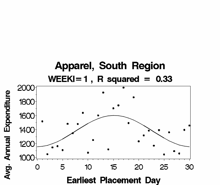
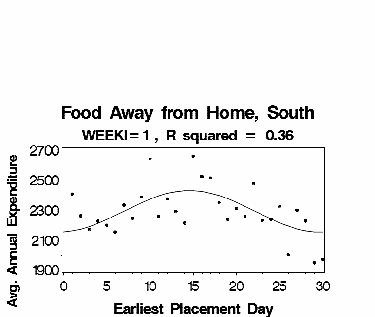
The only category that might have a consistent pattern is the South region where three of nine major groups have statistically significant R-squared values. Here are graphs of those three major groups – All Items, Apparel, and Food Away from Home. All of them have peak expenditures in the middle of the month which is an interesting feature. However, it is hard to explain why the South has statistically significant patterns but the other three regions do not, so again it seems likely these cycles are the result of normal random fluctuations in the data.
Conclusion
Clearly there are monthly cycles in the expenditures that respondents report on their weekly diaries – higher rent and utilities expenditures are reported on diaries that are placed near the beginning of the month, while higher expenditures on “Food Away from Home” are reported on diaries that are placed near the middle of the month. Under the survey’s current diary placement protocol diaries are placed with respondents uniformly throughout the month to make sure all of the peaks and troughs of the expenditure cycles are reflected in the data as well as everything in between. The purpose is to produce unbiased expenditure estimates for every item category.
However, as it was mentioned earlier, some UCCs have stronger monthly expenditure cycles than others, and many of the UCCs with stronger monthly cycles are taken from the Interview survey in the integration process and not from the Diary survey. This has caused some people to wonder whether placing diaries uniformly throughout the month is really that crucial.
The data analysis presented here shows that when the universe of Diary UCCs is limited to those that are used in the integration process, the monthly expenditure cycles are considerably weaker and may not even exist. In particular, the monthly cycle for the “All Items” category completely disappeared, and the monthly cycles for all nine major groups were so weak that they failed to achieve statistical significance. Whatever cycles were observed (e.g., “Apparel in the South” or “Food Away from Home in the South”) were probably the result of normal random fluctuations in the data that are expected in the survey’s data rather than actual expenditure cycles.
1 Except February 29 and July 4. No addresses are assigned to those days.
2 The cosine function is used instead of the sine function because its parameters are easier to interpret, especially the phase shift 2. Its period was pre-set to 30.4 days (the average number of days in a month) because we are interested in monthly cycles, not weekly or yearly cycles, and SAS had trouble figuring out the period on its own.
3 The distribution of the R-squared statistic was empirically determined by drawing 1,000,000 random samples from a N(0,1) normal distribution with n=31 observations per sample. A cosine function was fit to each sample generating 1,000,000 values of the R-squared statistic. The distribution’s 50th percentile was 0.050; its 75th percentile was 0.098; its 90th percentile was 0.157; its 95th percentile was 0.199; its 99th percentile was 0.289, its 99.5th percentile was 0.324; and its 99.9th percentile was 0.399. These results show that R-squared values over 0.30 are significant at the 0.01 level, and R-squared values over 0.20 are significant at the 0.05 level. Of course in real life data never have a N(0,1) normal distribution, so these numbers need to be taken with a grain of salt.
4 Most of the other 272 UCCs were taken from the Interview survey, although a few of them were not taken from either survey because they were non-expenditures like mortgage payments and saving account deposits, or because the two surveys had different UCC codes and their expenditures were taken from the Interview survey (e.g., magazines are UCC=590210 in Diary and UCC=590310/590410 in Interview, and they were taken from Interview so UCC=590210 was not taken from either survey). Also, the source of data in the integration process changes from time-to-time, and in this memo it was considered to be the Diary survey if the UCC was taken from that survey at any point in the 2009-2013 time period, else it was considered to be a non-Diary or non-expenditure UCC.
| File Type | application/vnd.openxmlformats-officedocument.wordprocessingml.document |
| Author | blswksta |
| File Modified | 0000-00-00 |
| File Created | 2021-01-23 |
© 2026 OMB.report | Privacy Policy