CHIPS Pre-Application Information Collection
CHIPS Pre-Application Information Collection
Financial Model White Paper vF. 8.4.23 docx
CHIPS Pre-Application Information Collection
OMB: 0693-0095
CHIPS Incentive Program – Commercial Fabrication Facilities
Pre-Application
Project Forecasting –
Example White Paper
Table of Contents
1. Overview 2
2. Control Panel Inputs & Assumptions 3
2.6. Project Financing Assumptions 8
2.8. Depreciation Assumptions 9
2.9. Working Capital Assumptions 10
3. Model Assumption Outputs (Assumptions Processing) 11
4. Depreciation Schedule 12
5. Outputs: Income Statement, Cash Flow Model, Balance Sheet 12
This document serves as a tool for potential applicants considering submitting a pre-application under the CHIPS Incentives Program-Commercial Fabrication Facilities Notice of Funding Opportunity (NOFO). This white paper and accompanying financial model tool have been created as an example of the “Summary Financials for Each Project” to be submitted as part of an optional pre-application per section IV.H.3 of the NOFO.
Disclaimer: Use of this CHIPS financial model tool is not a requirement for the CHIPS optional pre-application submission. Any materials submitted that fulfill the requirements of the “Summary Financials for the Project” portion of the Pre-Application is acceptable. The financial model is intended to act as an illustrative example of the level of granularity expected and may not appropriately meet the needs of all projects. It is a potential applicant’s responsibility to ensure its financial forecasts are suitable and accurate, and aligned with the requirements listed in Section IV.H.3 of the NOFO. Nothing in this White Paper or the model are intended to contradict the requirements in the CHIPS Incentives Program - Commercial Fabrication Facilities NOFO. Any conflicts must be resolved in favor of the NOFO.
The CHIPS financial model tool is generally structured in three main components:
Inputs: Data on key project assumptions are inputted in designated input fields in the “Control Panel” worksheet in the “Inputs” section
Processing: Using the information in the “Control Panel” worksheet, the model processes the key assumptions through processing worksheets (“Assumptions Processing” and “Depreciation Schedule”)
Outputs: These processing worksheets are used to produce model outputs in the form of an Income Statement, Balance Sheet, and Cash Flow Statement
Further, the CHIPS financial model tool has the following features:
The model is pre-populated with mock assumptions for an illustrative project. All pre-populated values are purely illustrative and intended to demonstrate how the model works, rather than provide any guidance on the magnitude or timing of assumptions.
The model contemplates certain simplifying assumptions. Applicants may want to reflect additional complexities in their materials.
The model uses an annual timestep and covers the entire expected life of an illustrative facility (including construction and operation phases); the life of the facility is assumed to be 20 years with year “1” reflecting the first year of the forecast and year “20” reflecting the final year.
The financial information in the model is all in U.S. dollars.
The tool features 7 worksheets grouped into four sections (“Inputs”, “Processing”, “Outputs”, and “Other”). The sections are described in the table below.
Table 1: CHIPS Financial Model Tool Contents
Worksheet |
|
Description |
Inputs >> |
Control Panel |
Main tab that controls assumptions and inputs |
Processing >> |
Assumptions Processing |
Helper worksheet to structure inputs for model outputs |
Depreciation Schedule |
Helper worksheet to calculate depreciation and investment tax credit |
|
Outputs >> |
Income Statement |
Model output summarizing income statement for the project |
Cashflow |
Model output summarizing a cash flow statement for the project |
|
Balance Sheet |
Model output summarizing a balance sheet for the project |
|
Other >> |
Drop-downs |
Helper worksheet to define options in tool’s drop downs |
The “Control Panel” worksheet is the source for all assumptions. It is the only worksheet that requires -user inputs.
In this worksheet there are three different types of cells, as described in the figure below.
Figure 1: Control Panel Legend

Direct input: Designated through a pale-yellow fill, the direct input cells contain no formulas and are where the model inputs and assumptions are provided
Interim calculation: Designated through grey italicized text, the interim calculations are cells that provide calculated values based on other values in the worksheet.
Cross sheet reference: Designated through a grey fill, the cross-sheet references reflect calculations pulled from other sheets in the workbook.
The control panel also contains an Error Checks section which helps to quickly identify issues with inputs. The Error Checks section contains three different types of checks, which are shown in the figure below.
Figure 2: Error Checks

Inputs: Checks to ensure that key inputs are consistent (e.g., total amount of initial capital investment spend across multiple years equals the total amount of invested capital)
Cash Balances: Checks to ensure that the cash balances are positive across all years in the forecast
Balance Sheet: Checks to ensure that the balance sheet reconciles (e.g., Assets = Liabilities + Equity)
The “Control Panel” assumption inputs are segmented into a series of themes throughout the tab. These themes are designated through a light blue line and reflect assumption groups (e.g., “Project Capital Costs” or “Debt Assumptions”). The following subsections provide an overview of each theme.
Section “(A) Overview” is where the project name can be defined. The financial model uses numbered years (e.g., 1-20) to delineate when an activity is occurring. For example, when a project capital cost is spread out equally over year 1 and year 2, half the cost will be incurred in the 1st year and half the cost will be incurred in the 2nd year.
The Capital Costs section of the “Assumptions” worksheet is used to enter details on the capital expenditures for the project.
In the example financial model, the capital costs for the section are segmented into two main types with different input assumptions for each:
Initial Capital Investment: These reflect the capital costs required to complete the construction, expansion, or modernization of the project and initiate operation. This includes land, construction, equipment, infrastructure improvements, and administrative expenses directly attributable to the construction, expansion, or modernization.
Ongoing Annual Capital Investment: These reflect capital costs that occur after the construction, expansion, or modernization portion of the project is completed and the facility is operating. These generally are expected costs around the replacement and upgrading of its capital investments (e.g., equipment maintenance / upgrades).
For initial capital investment, the model uses both the size and timing of the initial capital investment spend. For each cost type, the amount and timing of the expense is designated by providing a percentage value under each of the five “year” columns. The percentage reflects the percentage of the cost that is incurred in that year and the five years provided reflect the first five years of the project. The timing totals for each cost should sum up to 100%.
The “Total Initial Capital Investment” value is formulaically populated based on the inputs for each individual cost line.
In the example model, the initial capital investment can only be categorized under one of six categories: land, construction, equipment, administrative expenses, infrastructure improvements, and other capital investment. The model is only set up to measure these types of capital investments but applicants may have other types of initial capital costs that should be captured in their respective models.
Figure 3: Capital Costs - Initial Capital Investment

For ongoing annual capital investment, this example specifies:
Annual cost: The annual capital investment is sized as a percentage of the initial capital investment spend described above
Start year: The start year determines when in the forecast the annual capital investment begins
Applicants may want to set up their financials to show ongoing annual capital investment differently.
Figure 4: Capital Costs - Ongoing Capital Investment

Note: Interest / fees during construction and start-up working capital are not included as project costs. Interest, fees, and working capital are calculated in other sections. Interest will be addressed in section 3.5 and working capital will be addressed in section 3.9. Within the financial model, both of these sections are further down on the “Control Panel” under “Debt Assumptions” and “Working Capital Assumptions”.
The Project Revenue section of the “Assumptions” worksheet contains input cells required to calculate revenues generated by the project. The assumptions are as follows:
Unit production capacity, monthly: The number of wafers (or other facility output) expected to be sold from the facility each month at peak capacity. Although not built into the tool, as stated in the NOFO, the applicant should provide summary narrative of assumptions discussing how this number is estimated and may include discussion on facility utilization and production yields.
Unit price in first year of production: The expected price for units sold during the first year of production. The first year of production is determined by the “Start year” in the “Unit production ramp up” assumptions.
Unit price change: The annual price increase or decrease per unit. For simplicity, the example model assumes a single annual price change (here, a decline) over the lifetime of the product as a percentage of the prior year’s price. Applicants may want to reflect different annual assumptions in their models.
Unit production ramp up (% of total capacity): For simplicity, the model assumes a linear production ramp to full capacity from the start year to the end year. The start year is the year in which the first unit will be sold (i.e., Year 2 in this example as we anticipate selling units one year after construction begins) and the end year is the year in which the facility will reach full production capacity. Therefore, in the example model, capacity ramps over 3 years with the first year having 33.3% capacity (80,000 wafers), the second year 66.6% capacity and the last year, year 4, the facility is at full capacity (240,000 wafers). Applicants may want to reflect non-linear production ramps in their models.
Figure 5: Project Revenue Assumptions

The Operating Costs section of the “Assumptions” are structured with two main inputs:
Run rate cost: The run rate cost reflects the expected size (in USD) of a given operating cost at the time production is at full capacity (i.e., the “End year” of the “Wafer production ramp up” period). Production costs ramp linearly with production output. As above, applicants may want to reflect non-linear production cost ramp in their models.
Annual change after production ramp up: This column determines how the run rate assumptions change over time. A percentage value indicates how the costs will evolve over time as the project matures where a positive value means costs will increase, a negative value means costs will decline, and zero means costs remain the same.
The example financial model has been pre-populated with five common operating expense line items. Applicants may have different common operating expense line items in their respective models.
Materials / Consumables / Chemicals: Costs for materials, consumables, and chemicals (i.e., direct material inputs)
Labor: Costs for direct labor in unit production
Utilities: Costs for utilities
SG&A: Selling, general, and administrative costs
R&D: Research and development costs
Figure 6: Operating Cost Assumptions

The Debt Assumptions section of the “Assumptions” worksheet is used to enter key assumptions for the expected debt used to finance the project.
This section covers assumptions for up to two types of debt for a project (senior debt and subordinated debt). This model assumes that the senior and subordinated debt are both construction loans with multiple disbursements being made over the course of the construction and equipping phase of the facility. However, applicants may not have construction loans and disbursement may be made in the same year (loan disbursement start date is equal to loan disbursement end date).
Note that the debt assumptions are generic and do not differentiate between private debt and debt requested from the CHIPS program. For guidelines around CHIPS Loans and Loan Guarantees, please review Section I.B.8 of the NOFO.
The debt assumptions in the financial model have the following attributes:
Annual interest rate (%): The annual interest rate to be paid on the debt
Tenor (years): The number of years until the loan matures
Amortization start (year): The year in which the principal of the debt will begin to be repaid; note that in this model the principal payment cannot occur until after the loan has been fully disbursed. Therefore, the model requires that the “loan disbursement end” occurs before the “Principal Repayment start”.
Loan structure: Indicates whether the amortization schedule will be a bullet structure (i.e., entire principal is repaid at maturity) or a straight-line amortization structure (i.e., principal will be repaid in installments throughout the life of the debt)
Total loan amount: The total amount of the debt that is expected to be raised for the project
Loan disbursement start / end: The year in which disbursement of the debt will begin and the year in which the final disbursement of debt will be received. For simplicity, the model will disburse the loan evenly each year from the start year to the end year.
Figure 8: Debt Assumptions

The Project Financing Assumptions section of the “Assumptions” worksheet offers key assumptions for the expected size and timing of Equity and Grant Contributions to the project.
The Equity in the project can reflect any non-government equity that is used to fund the project. The grant contributions can reflect either CHIPS Direct Funding or other incentives received from States or local governments.
For the CHIPS Direct Funding and state and local incentives, the model specifies both the size and timing of the incentives. For the equity contributions, the value is automatically calculated as the funding difference between the initial project capital costs and other funding sources (debt and incentives).
Timing is indicated by providing a percentage value under each of the five “year” columns. The percentage reflects the percentage that is injected in that year. The five years provided reflect the first five years of the project.
To ensure that all costs are appropriately captured in the model, the timing totals for each sum up to 100%.
Figure 7: Project Financing Assumptions

The Tax Assumptions section of the “Assumptions” worksheet contains key assumptions concerning the taxes the project will pay. Importantly, this section also provides a rough example of how to size the benefit of the credit the project could receive from the Advanced Manufacturing Investment Credit (Investment Tax Credit or ITC) under Section 48D of the Internal Revenue Code. The calculations shown below are only an approximation of the tax benefit of the ITC. In the example model the tax benefit is framed as a series of percentages. However, it may be easier for applicants to simply calculate the estimated overall value of the ITC for their projects. This approximation of the tax credit is purely illustrative and is not intended to be, and should not be, relied upon by applicants. The actual application of the ITC will be subject to IRS rules and guidance and the specific applicant and project. Applicants should consult their tax advisors to model the treatment of the ITC based on their individual facts and circumstances. Inputs for this section are as follows:
Tax Rate: An tax rate intended to estimate all taxes the company may have to pay on earnings related to the facility
Investment Tax Credit (ITC) rebate: The estimated percentage of ITC earned on qualifying investments for the project. The ITC is only available for investments in qualified tangible property (not for other expenditures) made after August 9, 2023 as part of projects that begin construction before the cut-off date in 2026, and that are placed in service after 2022. Applicants should consult their tax advisors to ensure appropriate treatment of the ITC based on their individual projects.
% of Qualifying CapEx for ITC: The estimated percentage of the total capital expenditures that will qualify for the Investment Tax Credit. This assumption applies a straight percentage of the total capital expenditures, although the ITC is only available for investments in qualified tangible property (not for any other expenditures). Applicants should consult their tax advisors to model the percentage of qualifying CapEx applicable to their individual projects.
Figure 8: Tax Assumptions

The Depreciation Assumptions section of the “Assumptions” worksheet allows key assumptions concerning depreciation of the project’s property, plant, and equipment. Depreciation should be calculated in accordance with US Generally Accepted Accounting Principles (GAAP). Refer to the figure below to see an example of the input categories. These investment categories will be depreciated over the term provided in the box on a linear schedule (e.g., Construction depreciates over 15 years in a straight line). If the line item will not be depreciated, simply enter a zero for the input.
For each Capital Investment category, provide the expected number of years that investments in this category will depreciate
Construction
Equipment
Administrative Expenses directly attributable to facility construction
Infrastructure improvements
Other Capital Investment
Ongoing annual capital expenditures (after facility initiates operation)
Figure 9: Depreciation Assumptions

The Working Capital Assumptions section of the “Assumptions” worksheet allows key assumptions concerning working capital needed for the project.
For each working capital category, provide the estimated time requirement in days or months, where applicable. Working capital assumptions are tied to production, as production ramps the working capital lag begins to kick in.
Days in Receivables
Days Inventory
Days in Payables
Months Debt Service to Restricted Cash - The debt service reserve is a fund that is set aside to ensure that there are sufficient funds to meet debt obligations. The purpose is to act as a buffer against potential cash flow shortfalls for debt service
Figure 10: Working Capital Assumptions

The Excess Cash section of the “Assumptions” worksheet is used to enter key assumptions concerning any distributions.
An annual time series is provided with the period cash balance (calculated from the linked balance sheet) provided only as a reference.
Distribution: Model allows the specification of the year that distributions can begin and the minimum cash balance to be held. The tool requires that a minimum amount of cash be held for the project to be eligible to take a distribution. Based on these inputs, the tool will calculate a proposed distribution.
Figure 11: Distribution Assumptions

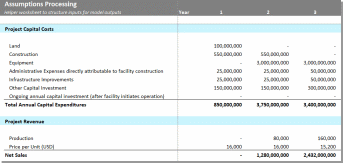
The “Assumptions Processing” worksheet is a processing worksheet that structures the inputs from the control panel to produce outputs in the financial statement.
Instructions:
This worksheet is entirely driven by the control panel; there are no inputs in this worksheet for the model to produce outputs
Figure 12: Assumptions Processing Tab
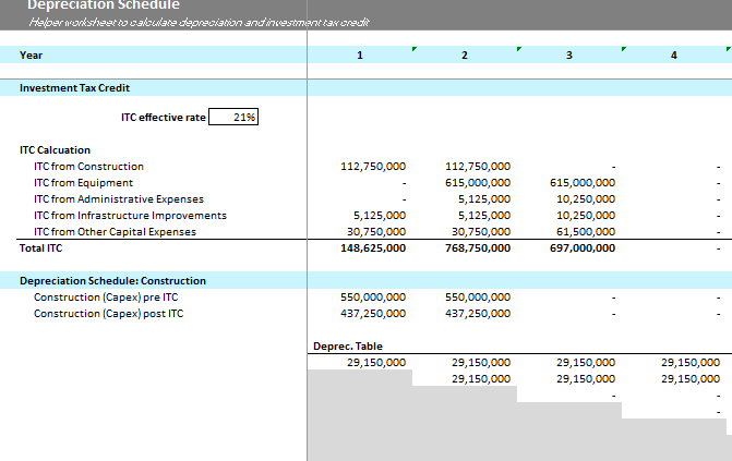
The “Depreciation Schedule” worksheet calculates the depreciation of the project’s capital costs and the estimates the benefit from the Investment Tax Credit (ITC).
All depreciation is calculated on a straight-line basis (i.e., the depreciation expense is equal across the depreciable life of the asset)
This worksheet is entirely driven by the control panel
Each applicant should show a depreciation schedule that accurately reflects its project
The ITC rebate is calculated by multiplying each of the capital investment types in a given year (e.g., construction year 1 investment) by (1 - effective ITC rate), and then subtracting that value from the original investment.
Figure 13: Depreciation Schedule and ITC Tab
The Financial model contains three output tabs, each summarizing a different financial statement. There are no inputs in any of these tabs and they are intended to act as reference outputs only. The sections below are designed to give an example of how these financial statements could be linked and presented.
The following sub-sections provide an overview of each worksheet.
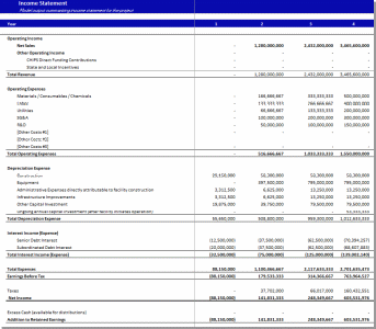
The “Income Statement” worksheet shows the income, or profit and loss, statement that has been generated using the assumptions entered on the “Control Panel” worksheet. This worksheet shows the revenues and operating expenses in absolute terms ($USD).
Figure 2: Project Income Statement
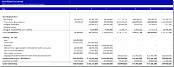
The “CashFlow” worksheet has three output sections.
The first section is the cash flow statement for the project.
The second is the debt service coverage analysis. This shows the project’s ability to pay debt service in each period.
The final section is the cash flow to equity which shows the cashflows for the equity position in the project. Equity investments reflect outflows for the equity holder from equity injections and equity payouts reflect cash inflows from the project to the equity holder.
Figure 15: Cash Flow for Project
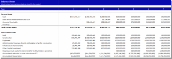
The “Balance Sheet” worksheet brings together all the flows, cash and non-cash, to show the “accumulation” of each type of asset and liability/equity at the end of each period.
Figure 16: Project Balance Sheet
| File Type | application/vnd.openxmlformats-officedocument.wordprocessingml.document |
| Author | Parcell, Jack |
| File Modified | 0000-00-00 |
| File Created | 2023-09-28 |
© 2026 OMB.report | Privacy Policy